Building a Bigram Character-Level Language Model

Introduction

Today, we will be building a Bigram Language Model which takes in a text file as training data and generates output text similar to the training data.

More specifically, this post is a step-by-step guide of Andrej Karpathy’s makemore project (Video Lecture). Makemore is a simple character-level language model that uses a neural network to predict the next character in a sequence. The example code takes in the names.txt file as training data and generates output texts that somewhat resemble names.

This post is a step-by-step guide of the code in the makemore project. I will be using Python and PyTorch to implement the code.

Bigram Language Model

A Bigram Language Model is a probabilistic language model that predicts the next word (or character) based on the previous one. The term bigram refers to a pair of consecutive elements (in our case, characters) from a sequence of text. A bigram is an n-gram for n=2.

For example, given the word “hello”:

• The bigrams would be: ('h','e'), ('e','l'), ('l','l'), ('l','o').
• For each character, the model learns the probability distribution of what character is likely to come next.
• When generating text, it uses these learned probabilities to predict the next character.

In the context of our character-level model:

• Input: A single character.
• Output: Probability distribution over all possible next characters.
• Training: Model learns these probabilities from the patterns in our training data (names.txt).

A mathematical representation of a bigram model is:

\[P(w_1, w_2, ..., w_n) = \prod_{i=1}^{n} P(w_i | w_{i-1}) = P(w_1) \cdot P(w_2 | w_1) \cdot P(w_3 | w_2) \cdot ... \cdot P(w_n | w_{n-1})\]

For example, given the word “hello”, the probability of the word is calculated as:

\[P(h, e, l, l, o) = P(h | \text{<S>}) \cdot P(e | h) \cdot P(l | e) \cdot P(l | l) \cdot P(o | l) \cdot P(\text{<E>} | o)\]

<S> and <E> are special start and end tokens that are added to the beginning and end of the sentence to indicate the start and end of the sentence. And we will be covering more about these in the following section of this post.

Dataset Overview

Before we start building the bigram language model, it is important to understand the dataset we are working with.

Downloading the Dataset

Using the requests library, we will directly download the names.txt file from the given URL and store it in the words array.

import requests

# Raw URL for the file
url = "https://raw.githubusercontent.com/karpathy/makemore/master/names.txt"

# Download and store names in a list
try:
    response = requests.get(url)
    response.raise_for_status()  # Raise an HTTPError for bad responses
    words = response.text.strip().split('\n')  # Split the content into a list of names
    print(f"File downloaded successfully. Total names: {len(words)}")
except requests.exceptions.RequestException as e:
    print(f"An error occurred: {e}")

Data Analysis

Following lines of code will help us understand:

• Verify the dataset is loaded correctly and what kind of data it contains.
• Verify the total number of names in the dataset.
• Verify the unique characters in the dataset.
• Verify the longest and shortest word in the dataset.

print(f"First 10 names: {words[:10]}")
# First 10 names: ['emma', 'olivia', 'ava', 'isabella', 'sophia', 'charlotte', 'mia', 'amelia', 'harper', 'evelyn']

print(f'total word counts: {len(words)}')
# total word counts: 32033

chars = sorted(list(set(''.join(words))))
print(f'unique characters counts: {chars}')
# unique characters counts: ['a', 'b', 'c', 'd', 'e', 'f', 'g', 'h', 'i', 'j', 'k', 'l', 'm', 'n', 'o', 'p', 'q', 'r', 's', 't', 'u', 'v', 'w', 'x', 'y', 'z']

longest_word = max(words, key=len)
print(f'longest word: {longest_word, len(longest_word)}')
# longest word: ('muhammadibrahim', 15)

shortest_word = min(words, key=len)
print(f'shortest_word: {shortest_word, len(shortest_word)}')
# shortest_word: ('an', 2)

Building a Bigram Language Model

We will be building a bigram language model using two different approaches:

1. Statistical Approach
   • Uses the frequency of each character pair to calculate the probability of the next character.
2. Neural Network Approach
   • Uses a neural network to learn the probability of each character pair.

Prerequisite: Understanding Special Tokens in Tokenizers

Although we have not covered the concept of tokens or tokenizers yet, our implementation of bigram language model will be using a simple special token (e.g., .) to indicate the start and end of the word.

We will be covering the concept of tokens and tokenizers in depth in a later post. For now, let’s briefly cover the concept of tokenizer and special tokens.

Tokenizer

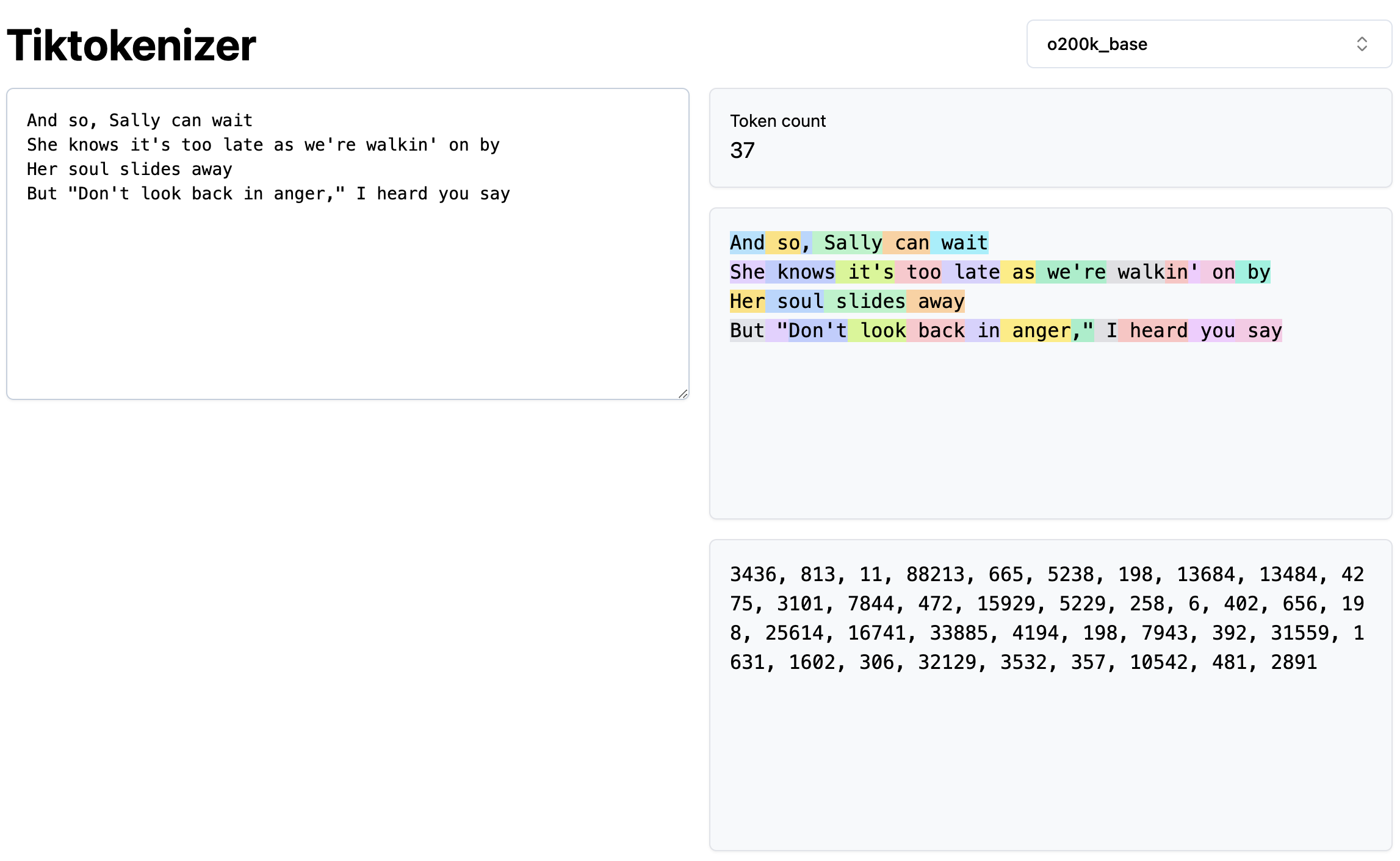
A tokenizer is a tool that breaks down text into smaller units called tokens. These tokens are the basic building blocks of any NLP model.

From the picture below, we can see that the tokenizer breaks down the text into smaller units called tokens.

Special Tokens

Special Tokens in tokenizers are reserved tokens that serve specific purposes in natural language processing (NLP) models.

You can see the example of gpt-3.5-turbo’s special tokens (e.g., |im-start| and |im-end|) in the picture below.

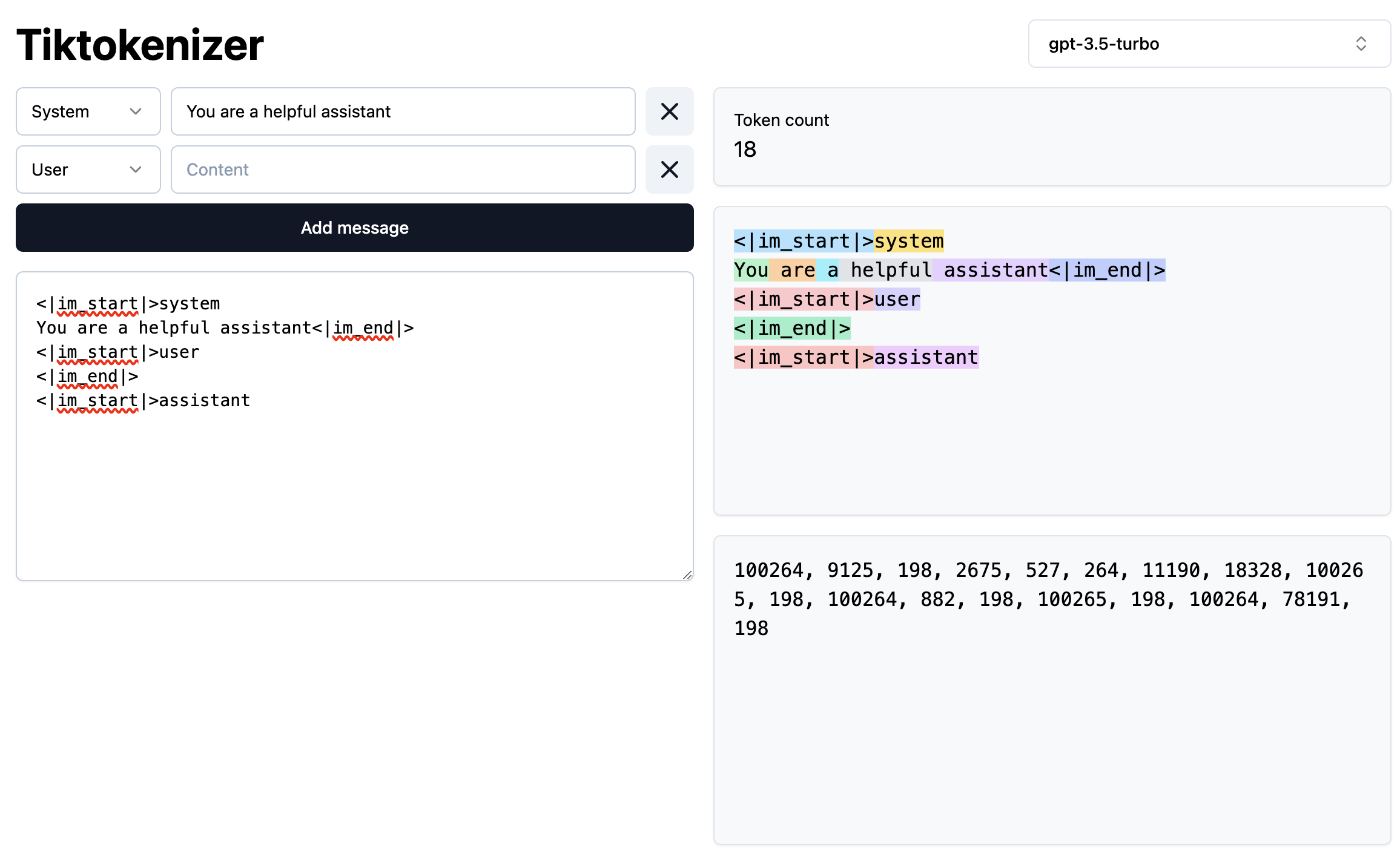
Special tokens differ by model; however, they have the same purpose: to provide additional context or control to the model. Common special tokens include:

• [START]/[END]: Mark the beginning and end of sequences
• [PAD]: Used for padding sequences to a fixed length
• [UNK]: Represents unknown tokens not in the vocabulary
• [MASK]: Used in masked language modeling tasks
• [SEP]: Separates different segments of text
• [CLS]: Used for classification tasks

In our bigram model implementation, we’ll use a simple '.' token to mark both the start and end of words.

Statistical Approach

From the previous section, we have verified that the dataset is composed of 26 unique lowercase alphabets. And since we are building a bigram language model, we will be using the frequency of each character pair to calculate the probability of the next character.

If you recall the mathematical representation of a bigram model, we need to calculate the probability of each character pair. This can be done by:

• Counting the frequency of each character pair in the dataset.
• Then normalizing the frequency by the total number of character pairs.

Counting the Frequency of Each Character Pair

The code below creates a list of unique sorted characters from the dataset and maps each character to an index (i.e., stoi). Then it inverts the mapping to create a list of characters from the index (i.e., itos). Finally, we create a 27x27 matrix N to store the frequency of each character pair.

import torch # make sure to install torch before importing

chars = sorted(list(set(''.join(words))))

stoi = {char: idx+1 for idx, char in enumerate(chars)}
stoi['.'] = 0 # Special token for start and end of the sentence

itos = {v: k for k, v in stoi.items()}

N = torch.zeros((27, 27), dtype=torch.int32)

for w in words:
    # Special Token: '.' denotes START or END of the context
    context = ['.'] + list(w) + ['.']

    for ch1, ch2 in zip(context, context[1:]):
        ix1 = stoi[ch1]
        ix2 = stoi[ch2]

        N[ix1, ix2] += 1

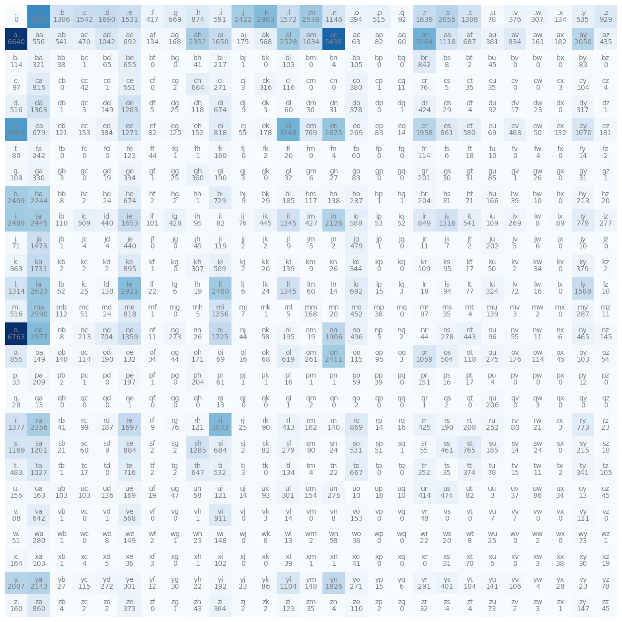
The visualization below shows the frequency of each character pair is stored in the matrix N. This helps us understand pairs such as ('.', 'a'), ('a', '.'), ('a', 'n'), ('n', '.') and ('a', 'r') have high frequency.

import matplotlib.pyplot as plt
%matplotlib inline

plt.figure(figsize=(16,16))
plt.imshow(N, cmap='Blues')
for i in range(27):
    for j in range(27):
        chstr = itos[i] + itos[j]
        plt.text(j, i, chstr, ha="center", va="bottom", color='gray')
        plt.text(j, i, N[i, j].item(), ha="center", va="top", color='gray')
plt.axis('off');

Normalizing the Frequency

We can not use the raw count of each character pair to calculate the probability of the next character. Instead, we will normalize each row by dividing each frequency by the total number of character pairs in the row.

Broadcasting

We have covered the concept of broadcasting in the previous post. In this case, we are using broadcasting to normalize the frequency of each character pair:

• P is a 27×27 matrix (representing probabilities for each character pair)
• N.sum(1, keepdims=True) creates a 27×1 matrix (sum of each row)
• PyTorch automatically “broadcasts” the 27×1 divisor to match the 27×27 shape of P
• Each element in a row of P is divided by the corresponding row sum
• This effectively normalizes each row so they sum to 1

P = (N+1).float() # TODO: Apply model smoothing
P /= N.sum(1, keepdims=True) # Normalize the probability

From the diagram below, we can see that the probability of each character pair is correctly normalized (i.e., each row sums to 1, and the colors of each cell are consistent with the frequency of the character pair).

plt.figure(figsize=(16, 16))
plt.imshow(N, cmap='Blues')
for i in range(27):
    for j in range(27):
        chstr = itos[i] + itos[j]
        plt.text(j, i, chstr, ha="center", va="bottom", color='gray')
        plt.text(j, i, f"{P[i, j].item():.2f}", ha="center", va="top", color='gray')
plt.axis('off')

Sampling from the Bigram Model

Code below generates 5 random names from the bigram model. It starts with the special token '.' and iteratively samples the next character based on the probability distribution of the current character. The process continues until the special token '.' is sampled again, indicating the end of the word.

The first generated output iome is generated by (instead of using the probability distribution by checking the matrix P, we will be using a better evaluation method in the next section):

• Current character '.' samples a pair '.i' with probability of 2%.
• Current character pair '.i' samples 'io' with probability of 3%.
• Current character pair 'io' samples 'om' with probability of 3%.
• Current character pair 'om' samples 'me' with probability of 12%.
• Current character pair 'me' samples 'e.' with probability of 20%.

g = torch.Generator().manual_seed(1234567890) # Set the seed for reproducibility

for _ in range(5):
    ix = 0
    output = []

    while True:
        p = P[ix] # probability vector of current char
        ix = torch.multinomial(p, num_samples=1, replacement=True, generator=g).item() # draw with replacement
        output.append(itos[ix])

        if ix == 0:
            break
    print(''.join(output))

Even though the model is trained on the names.txt file, the generated names are not necessarily names (Karpathy’s reaction to the output is quite interesting). The bigram model, while simple and effective in certain scenarios, has inherent limitations that make it unsuitable for generating high-quality outputs like realistic names

iome.
ko.
anorll.
danie.
mezan.

Evaluating the Bigram Model Using the Loss Function

Now that we have trained a bigram model, we can evaluate the model using the loss function. The loss function is a measure of how well the model is performing. The lower the loss, the better the model is performing.

We will be using the negative log-likelihood (NLL) as the loss function. If you are not familiar with the concept of maximum likelihood estimation or negative log-likelihood, please refer to the post for more information.

log_likelihood = 0.0
n = 0

for word in words:
    context = ['.'] + list(word) + ['.']

    for ch1, ch2 in zip(context, context[1:]):
        ix1 = stoi[ch1]
        ix2 = stoi[ch2]

        prob = P[ix1, ix2]
        log_prob = torch.log(prob)
        log_likelihood += log_prob
        n += 1

        # print(f'{ch1}{ch2}: {prob:.4f} {log_prob:.4f}')

print(f'{log_likelihood=}')
nll = -log_likelihood
print(f'{nll=}')
print(f'{nll/n}')

The average negative log-likelihood (NLL) of 2.454 suggests our model is learning meaningful patterns from the training data. To put this in perspective:

• If our model was making completely random guesses (assigning equal probability of 1/27 to each character), we would expect an NLL of log(27) ≈ 3.29
• Our lower NLL of 2.454 indicates the model has learned useful character transition probabilities from the frequency matrix P

log_likelihood=tensor(-559891.7500)
nll=tensor(559891.7500)
2.454094171524048

Karpathy provides a nice summary of the evaluation process:

• Maximize likelihood of the data with respect to model parameters (statistical modeling)
• Equivalent to maximizing the log likelihood (because log is monotonic)
• Equivalent to minimizing the negative log likelihood
• Equivalent to minimizing the average negative log likelihood
  • $\log(a \cdot b \cdot c) = \log(a) + \log(b) + \log(c)$

Model Smoothing

Let’s say we are evaluating how much probability the model assigns to the word 'andrejq'.

for word in ['andrejq']:
    context = ['.'] + list(word) + ['.']

    for ch1, ch2 in zip(context, context[1:]):
        ix1 = stoi[ch1]
        ix2 = stoi[ch2]

        prob = P[ix1, ix2]
        log_prob = torch.log(prob)
        
        print(f'{ch1}{ch2}: {prob:.4f} {log_prob:.4f}')

Probability of jq is 0.0000 which assigns -inf to its log probability. This is because the model has not seen the character pair jq in the training data. In order to fix this, we can apply model smoothing.

.a: 0.1377 -1.9829
an: 0.1605 -1.8296
nd: 0.0384 -3.2594
dr: 0.0771 -2.5620
re: 0.1336 -2.0127
ej: 0.0027 -5.9171
jq: 0.0000 -inf
q.: 0.1029 -2.2736

Model smoothing is a technique used to handle unseen character pairs by adding a small amount of probability mass to all character pairs. This helps the model make more reasonable predictions even for unseen combinations.

If you are not familiar with the concept of model smoothing, I have a post which briefly covers the concept.

P = (N+1).float()

# after applying model smoothing of (N+1)
.a: 0.1377 -1.9827
an: 0.1605 -1.8294
nd: 0.0385 -3.2579
dr: 0.0773 -2.5597
re: 0.1337 -2.0122
ej: 0.0027 -5.8991
jq: 0.0003 -7.9725
q.: 0.1066 -2.2385

Neural Network Approach

This time, we will be taking an alternative approach to build a bigram language model using a neural network. Previously, the objective of the bigram model was to maximize the likelihood (or in other words, minimize the negative log-likelihood) with respect to the model parameters.

The model parameters were pre-calculated probabilities of each character pair stored in the matrix P. However, this time, we will be using a neural network to calculate the parameters (therefore the parameters or weights of the neural network (i.e., matrix W) will be initially set to random numbers).

In the neural network framework:

• The model will still accept a single character as input and output the probability distribution of the next character.
• The model parameters are the weights of the neural network (i.e., W).
• The model will be trained to minimize the loss function (i.e., negative log-likelihood) with respect to the model parameters.

Quick Overview: Neural Network

Our neural network will be a simple feedforward neural network with one hidden layer of size 27. The input layer will be a single character, and the output layer will be a probability distribution over all possible characters.

The diagram below shows the expected input and output of the neural network for a bigram pair of (".", "e").

Input

Since we can not pass in a single character to the neural network, we will be using the one-hot encoding to represent the input character. For example, the input character "." which has index 0 will be represented as:

• [1, 0, 0, 0, 0, 0, 0, 0, 0, 0, 0, 0, 0, 0, 0, 0, 0, 0, 0, 0, 0, 0, 0, 0, 0, 0, 0].

Hidden Layer

A hidden layer will be a 27×27 matrix W which will be initialized to random numbers. The matrix W will be used to calculate the hidden layer output.

Output

The output of the neural network will be a probability distribution over all possible characters. In this case, the output will be a 27×1 vector where the element at index 5 (which corresponds to the character "e") will be the highest.

Create a Dataset

Before training our neural network, we need to create a dataset of input-output pairs.

Each pair consists of:

• xs: An index-encoded current character
• ys: An index-encoded next character

For example, for the word “emma”, we create the following pairs:

• (".", "e") → (0, 5)
• ("e", "m") → (5, 13)
• ("m", "m") → (13, 13)
• ("m", "a") → (13, 1)
• ("a", ".") → (1, 0)

# create a dataset
xs = []
ys = []

for word in words:
    context = ['.'] + list(word) + ['.']

    for ch1, ch2 in zip(context, context[1:]):
        ix1 = stoi[ch1]
        ix2 = stoi[ch2]

        xs.append(ix1)
        ys.append(ix2)

xs = torch.tensor(xs)
ys = torch.tensor(ys)
num = xs.nelement()
print(f'num example: {num}')
print(f'xs[:5]: {xs[:5]}')
print(f'ys[:5]: {ys[:5]}')

num example: 228146
xs[:5]: tensor([ 0,  5, 13, 13,  1])
ys[:5]: tensor([ 5, 13, 13,  1,  0])

Input & Weight Matrix Initialization

g = torch.Generator().manual_seed(2147483647)
W = torch.randn((27, 27), requires_grad=True, generator=g).float()

import torch.nn.functional as F

xenc = F.one_hot(xs, num_classes=27).float()
print(f"xenc shape: {xenc.shape}")

xenc shape: torch.Size([228146, 27])

• Weight Matrix Initialization
  • W is our weight matrix of size 27×27 initialized with random numbers from a normal distribution using randn.
  • requires_grad=True: PyTorch tracks gradients for this tensor during backpropagation.
• Input Encoding
  • Converts our input indices into one-hot encoded vectors.
  • Each input character is represented as a vector of size 27 (one position is 1, rest are 0).
  • Processes all 228,146 examples at once (batch processing).
• Batch Processing
  • Instead of training one example at a time, we process all 228,146 examples simultaneously.
  • This vectorized approach is much more efficient than processing examples one by one.

The neural network will learn to adjust the weights in W to minimize the loss function, effectively learning the probability distributions for character transitions that we previously calculated manually in the statistical approach.

Training Loop

for epoch in range(100):
    # forward pass
    logits = xenc @ W # (228146, 27) @ (27, 27) = (228146, 27)
    counts = logits.exp()
    probs = counts / counts.sum(1, keepdims=True) # softmax
    loss = -probs[torch.arange(num), ys].log().mean() + 0.01*(W**2).mean() # negative log-likelihood

    # backward pass
    W.grad = None
    loss.backward()

    # update parameters
    lr = 50 # learning rate
    W.data += -lr * W.grad

    if (epoch+1) == 1 or (epoch+1) % 10 == 0:
        print(f"{epoch+1} : {loss.item()}")

1 : 3.7686190605163574
10 : 2.7188303470611572
20 : 2.5886809825897217
30 : 2.5441696643829346
40 : 2.522773265838623
50 : 2.5107581615448
60 : 2.503295421600342
70 : 2.498288154602051
80 : 2.494736433029175
90 : 2.492116689682007
100 : 2.4901304244995117

• Forward Pass
  • Matrix multiplication between one-hot encoded inputs and weights produces logits.
  • Softmax calculation converts logits to probabilities using:
    • Exponentiation (exp()) to make all values positive.
    • Division by row sums (using broadcasting) to normalize probabilities.
    • Each row sums to 1, representing probability distribution over next characters.
• Loss Calculation
  • Main loss: Negative log-likelihood (NLL) of correct next characters.
  • Regularization Term: L2 regularization (0.01*(W**2).mean()):
    • To read more about regularization techniques, please refer to my post.
    • Helps prevent overfitting by penalizing large weights.
    • λ=0.01 controls regularization strength.
• Backward Pass
  • loss.backward() computes gradients for all tensors with requires_grad=True.
  • Make sure to set grad to zero to avoid gradient accumulation.
• Parameter Update (Gradient Descent)
  • Updates weights using gradient descent: $W_t = W_{t-1} - \eta \cdot \frac{\partial L}{\partial W}$.
  • Learning rate (lr=50) controls the step size of updates:
    • 50 is a large learning rate compare to the normal neural network setting (e.g., 0.001 or 0.01). This is possible in this case due to well-behaved loss landscape.

After 20 epochs, the loss converges value close to 2.50, which is similar to the statistical model’s 2.45.

Sampling from the Neural Network Model

The sampling process is conceptually similar to our statistical approach, but instead of directly looking up probabilities in the P table, we:

1. Convert the current character index to a one-hot encoded vector
2. Use our trained neural network (matrix W) to compute probabilities
3. Sample the next character based on these probabilities

g = torch.Generator().manual_seed(1234567890) # Set the seed for reproducibility

for i in range(5):
    output = []
    ix = 0

    while True:
        xenc = F.one_hot(torch.tensor([ix]), num_classes=27).float()
        logits = xenc @ W 
        counts = logits.exp()
        probs = counts / counts.sum(1, keepdims=True)

        ix = torch.multinomial(probs, num_samples=1, replacement=True, generator=g).item()
        output.append(itos[ix])

        if ix == 0:
            break
    print(''.join(output))

iome.
ko.
anorll.
danie.
mezpghimannan.

Conclusion

In this post, we explored two different approaches to building a bigram language model:

• Statistical Bigram Model
• Neural Network Bigram Model

While both methods achieved similar results (NLL of ~2.45 for statistical and ~2.50 for neural network), they took fundamentally different paths to get there:

• Statistical Approach: directly calculates probabilities from frequency counts in a lookup table.
• Neural Network Approach: learned these probabilities through gradient descent on its weight matrix.

One key advantage of the neural network approach is its scalability. Consider extending this to a trigram model (predicting based on the previous two characters) or even larger n-grams:

• Statistical Approach: The size of the probability table grows exponentially (27³ for trigrams, 27⁴ for 4-grams, etc.)
• Neural Network Approach: The architecture can be adapted with minimal increase in parameters

This scalability advantage makes neural networks the preferred choice for more complex language modeling tasks, even though both approaches perform similarly for this simple bigram case.

Resources

• The spelled-out intro to language modeling: building makemore