Convolution Operation Explained

Side Note

While initially intended as an introduction to Convolutional Neural Networks (CNNs), I realized that a thorough understanding of the convolution operation itself is essential. This post therefore focuses on explaining the fundamental concept of convolution, serving as a foundation for future discussions about CNNs.

Introduction

Convolutional Neural Networks (CNNs) are a specialized class of neural networks designed to process and analyze visual data. Unlike fully connected networks, CNNs learn spatial hierarchies of features through the use of filters (also known as kernels), which slide across the input data to detect patterns such as edges, textures, and shapes.

These filters are typically much smaller than the input itself, and through repeated convolution operations, the network gradually learns to recognize increasingly complex and abstract features. By preserving the spatial structure of the data, CNNs excel at capturing local and global patterns in images.

Thanks to this ability, CNNs have become the de facto standard in computer vision and image processing tasks—from digit recognition to facial detection, object classification, and beyond.

In this article, we’ll explore how CNNs work, layer by layer, and understand why they’re so powerful for visual understanding.

Why Not Use Fully Connected Neural Network (FFNN)?

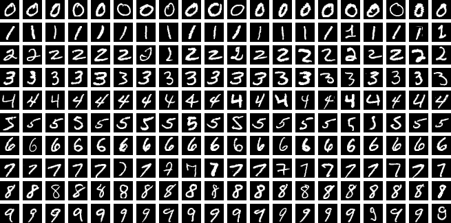
Imagine you are building a neural network to classify handwritten digits. Based on what we have learned so far, this might seem straightforward. Images can be represented as numerical data (with pixel values normalized between [0, 1]), and we can feed this data into a fully connected neural network (FFNN) just as we’ve done with other problems—like XOR classification. The typical process for classifying a 28x28 pixel image using a FFNN looks like this:

• Flatten the 2D image into a 1D input vector of shape (784, 1)
• Construct one or more hidden layers between the input and output layers
• Train the network by adjusting its parameters via backpropagation
• Use a softmax function on the output layer to produce probabilities for digit classification

However, fully connected neural networks have several critical limitations that make them less suitable for image processing tasks:

• Scalability Issues: FFNNs require a large number of parameters. For example, an image with 1024x1024 pixels would result in 1,048,576 input neurons—even before considering any hidden layers. This makes training inefficient and computationally expensive.
• Lack of Local Connectivity: In a FFNN, every neuron in one layer is connected to every neuron in the previous layer, regardless of spatial relevance. This results in many redundant connections and fails to take advantage of localized patterns in the image.
• Loss of Spatial Information: Since the image is flattened into a 1D vector, the network loses critical spatial relationships between pixels:
  • Would the network recognize the same digit if the image were slightly shifted to the left or right?
  • Pixel values in images are often spatially correlated—in MNIST, for instance, black pixels that make up digits tend to be clustered together, as do white background pixels. Flattening disrupts this structure.

These limitations motivate the use of Convolutional Neural Networks (CNNs), which are designed to efficiently capture spatial hierarchies and local patterns in image data.

What is a Convolution?

3Blue1Brown — "But What Is a Convolution?"

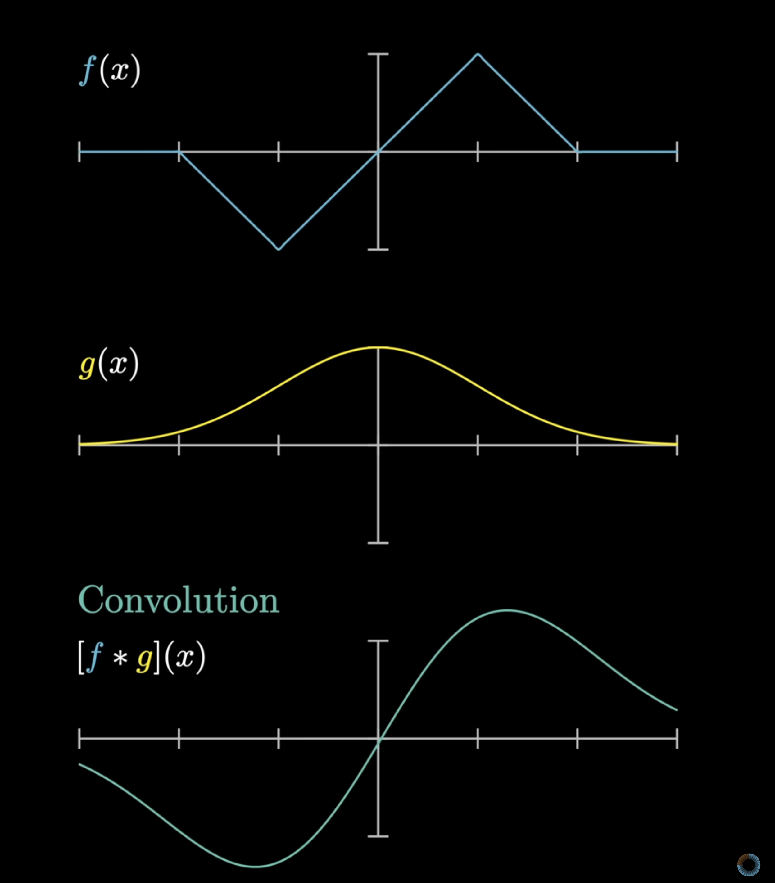
In mathematics, convolution is a mathematical operation that combines two functions, $f$ and $g$, to produce a third function $f * g$. The operation involves:

1. Reflecting one function (typically $g$) about the y-axis
2. Shifting the reflected function
3. Computing the integral of the product of the two functions

Convolution includes both the process of:

• Processing the computation by reflecting and shifting the function
• Computing the third function based on the alignment of two functions

In signal processing, convolution answers a practical question:

Given a signal $f(t)$ entering a linear-time-invariant (LTI) system with impulse response $g(t)$, what is the output $(fg)(t)$?*

The diagram below gives an intuitive understanding of time-domain convolution of input signal and kernel.

Mike X Cohen — "Convolution in the time domain"

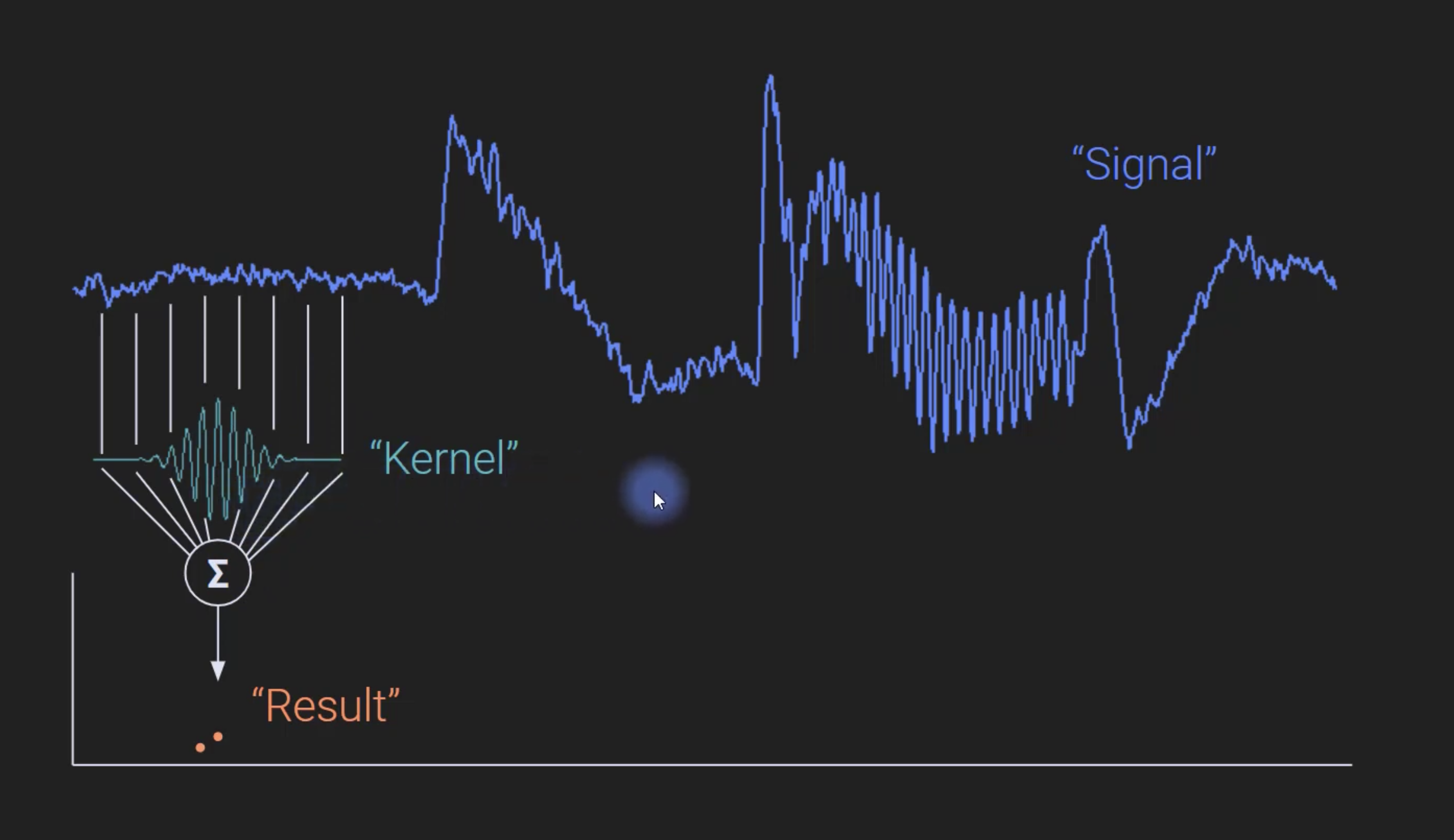
To compute the convolution at $t = 2$, we slide the kernel along the input signal, with the exact behavior at the edges determined by our padding strategy. At each position, we multiply the kernel values with their corresponding input values and sum the products to produce a single output sample.

Mike X Cohen — "Convolution in the time domain"

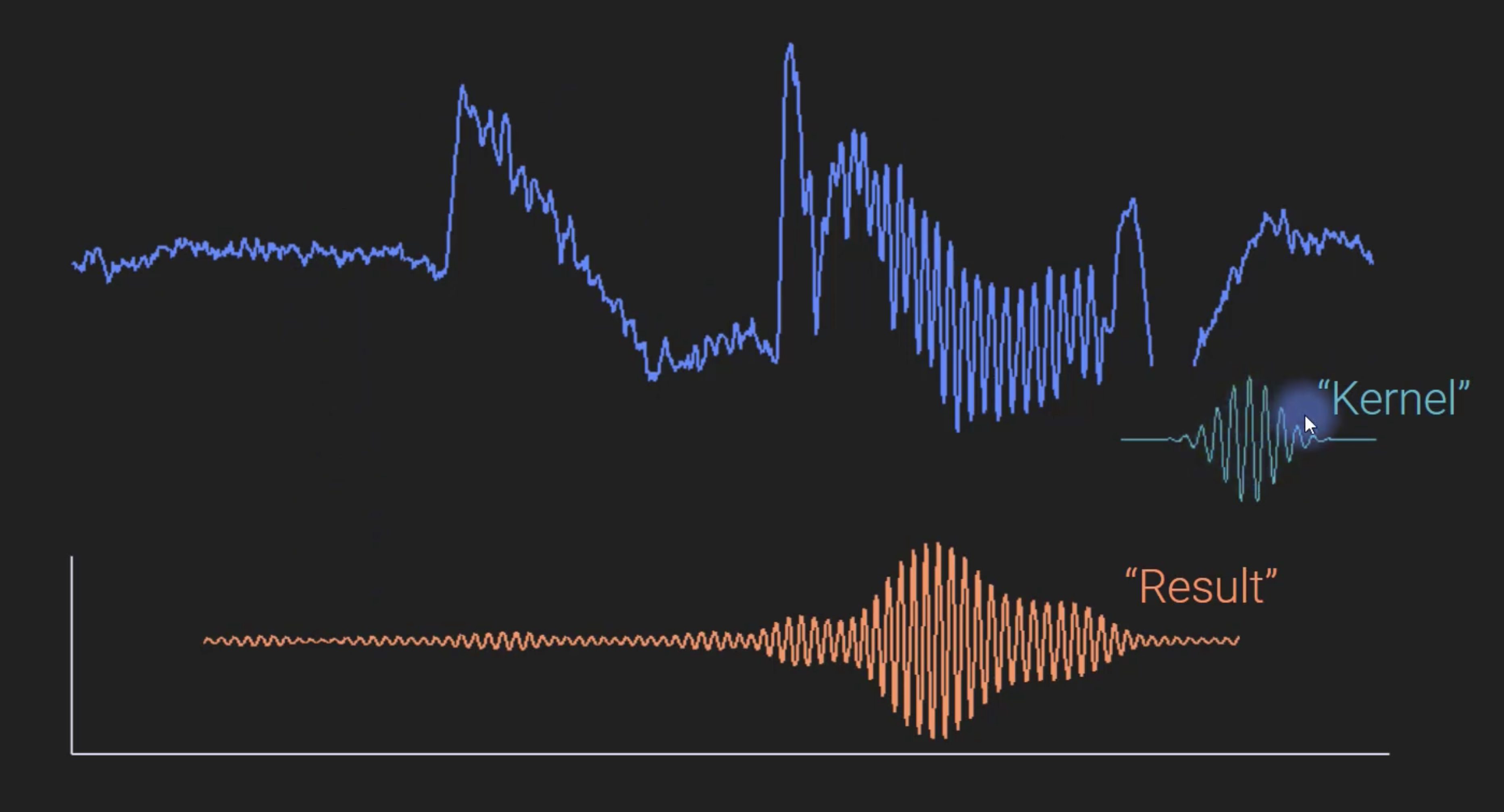
We repeat this sliding and multiplication process across the entire input signal, with the kernel’s position at each step determined by our chosen padding strategy. The final output is a new signal that represents how the input has been modified by the kernel at each point in time.

Continuous-time Definition:

\[(f * g)(t) \;=\; \int_{-\infty}^{\infty} f(\tau)\, g(t - \tau)\, d\tau,\; t \in \mathbb{R}.\]

Where:

• $t$: the moment at which you want the output
• $\tau$: a dummy variable that slides along the input
• $h(t-\tau)$: a time-reversed and shifted copy of $h$

Discrete-time Definition:

\[(x * h)[n] = \sum_{m=-\infty}^{\infty} x[m]\,h[n-m],\; m \in \mathbb{Z}.\]

The symbols change (sums instead of integrals) but the flip-shift-sum idea is identical.

Key Takeaways

• As functions, $f$ and $g$ map inputs to outputs, and their interplay allows us to describe the phenomenon at hand.
• $t$ is the unit of expressing both the inputs and outputs of the functions. For the convolution equation above, as we are trying to describe the phenomemon in terms of the changing time, we pass in $t$.
• The final output of $f$ and $g$ are mapped in each point $t$. We can use integral if we are interested in the output through out a continous domain.
• $\tau$ is parameter between function $f$ and $g$.
• The choice of which function is reflected and shifted before the integral does not change the integral result.

Why Flip the Kernel?

The term $h(t-\tau)$ (or $h[n-m]$) reverses the kernel and shifts it so that its origin aligns with the evaluation point $t$ (or $n$). This guarantees causal alignment: the input sample at time $\tau$ meets the kernel value located exactly $(t-\tau)$ seconds (or samples) later.

Example of Convolution

“..the beloved convolution formula that befuddles generations of students because the impulse response seems to be ‘flipped over’ or running backwards in time”

The quote above is from one of the most voted responses from StackExchange. Convolution can still be tricky even after looking at the mathematical equation (at least it was for me!) so let us go through an example to have a better grasp of it.

Below are the three resources that I found particularly useful understanding the operation:

• Convolution in the time domain
• Signal Processing: Flipping the Impulse Response in Convolution
• Intuitive Understanding of Convolution

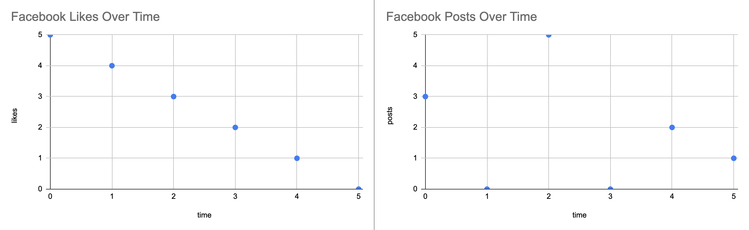
Left Chart

• Chart on the left shows the numbers of likes each post gets over time (hour). So when someone makes a post, he or she immediately gets 5 likes, 4 likes after an hour, and eventually 0 likes after 5 hours.

Right Chart

• Chart on the right shows the number of posts a social media team at Contoso posts during their work hours. They upload different number of posts during the day.

In this example, we can model the relationship between posts and likes using two time-dependent functions:

• $f(t)$: The posting rate function that describes how many posts are made at time $t$
• $g(t)$: The engagement function that describes how many likes a post receives $t$ hours after it’s published
• $(f*g)(t)$: The convolution of these functions, which gives us the total number of likes at any time $t$, taking into account both the posting schedule and the engagement pattern

The table reveals that the team’s like count at any given moment is the sum of fresh likes arriving now plus the lingering likes still trickling in from earlier posts. In short, likes accumulate over time and that cumulative nature is precisely what the convolution captures. Now, let’s compute the convolution output at different times:

• $(f*g)(1) = 12$
  • Likes received by 3 posts at $t=0$ = $12$ (3 posts × 4 likes per post after 1 hour)
• $(f*g)(4) = 28$
  • Likes received by 3 posts at $t=0$ = $3$ (3 posts × 1 like per post after 4 hours)
  • Likes received by 5 posts at $t=2$ = $15$ (5 posts × 3 likes per post after 2 hours)
  • Likes received by 2 posts at $t=4$ = $10$ (2 posts × 5 likes per post at posting time)
• $(f*g)(6) = 15$
  • Likes received by 5 posts at $t=2$ = $5$ (5 posts × 1 like per post after 4 hours)
  • Likes received by 2 posts at $t=4$ = $6$ (2 posts × 3 likes per post after 2 hours)
  • Likes received by 1 post at $t=5$ = $4$ (1 post × 4 likes per post after 1 hour)
• $(f*g)(8) = 4$
  • Likes received by 2 posts at $t=4$ = $2$ (2 posts × 1 like per post after 4 hours)
  • Likes received by 1 post at $t=5$ = $2$ (1 post × 2 likes per post after 3 hours)
• $(f*g)(9) = 1$
  • Likes received by 2 posts at $t=4$ = $0$ (2 posts × 0 likes per post after 5 hours)
  • Likes received by 1 post at $t=5$ = $1$ (1 post × 1 like per post after 4 hours)

Using this example, we have a better understanding of convolution operation:

1. We have two time-varying functions:
   • $f(t)$: The number of posts made at time $t$
   • $g(t)$: The number of likes a post receives after $t$ hours
2. The convolution $(f*g)(t)$ gives us the total number of likes at any given time $t$ by:
   • For each past time point $\tau$, multiply the number of posts made at $\tau$ by the number of likes those posts would receive at time $t$ (which is $t-\tau$ hours after they were posted)
   • Sum up these products for all possible values of $\tau$

This is why convolution is particularly useful for analyzing systems where:

• The input (posts) has a time-varying nature
• The system’s response (likes) has a temporal spread
• We need to track the cumulative effect over time

So Again, Why Flip the Kernel?

Okay, so far so good. The example clearly explains how the convolution operation captures the accumulative characterstic of combining functions $f$ and $g$. However, we can take a step further to gain intuition behind “flipping”.

Graphical Example

The Facebook examle above described the functions $f$ and $g$ in discrete time steps where we could easily calculate the total likes of published posts at specific hours. However, in many real-world scenarios, we need to work with continuous-time signals. Let’s modify our social media diagrams to work with continuous functions:

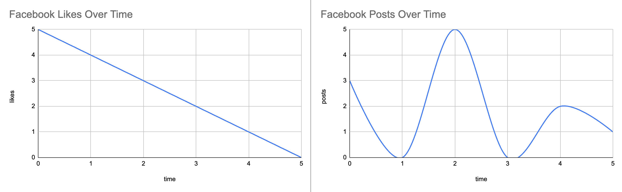
When we move from discrete to continuous time, we discover that integrating this product yields the overall output. In the discrete case, linking each input to its corresponding output is straightforward. In the continuous case, however, the input varies without interruption, making it much harder to describe the output produced at every instant. How, then, can we represent inputs and outputs more effectively for continuous time?

This is where reflection (flipping) and shifting come into play.

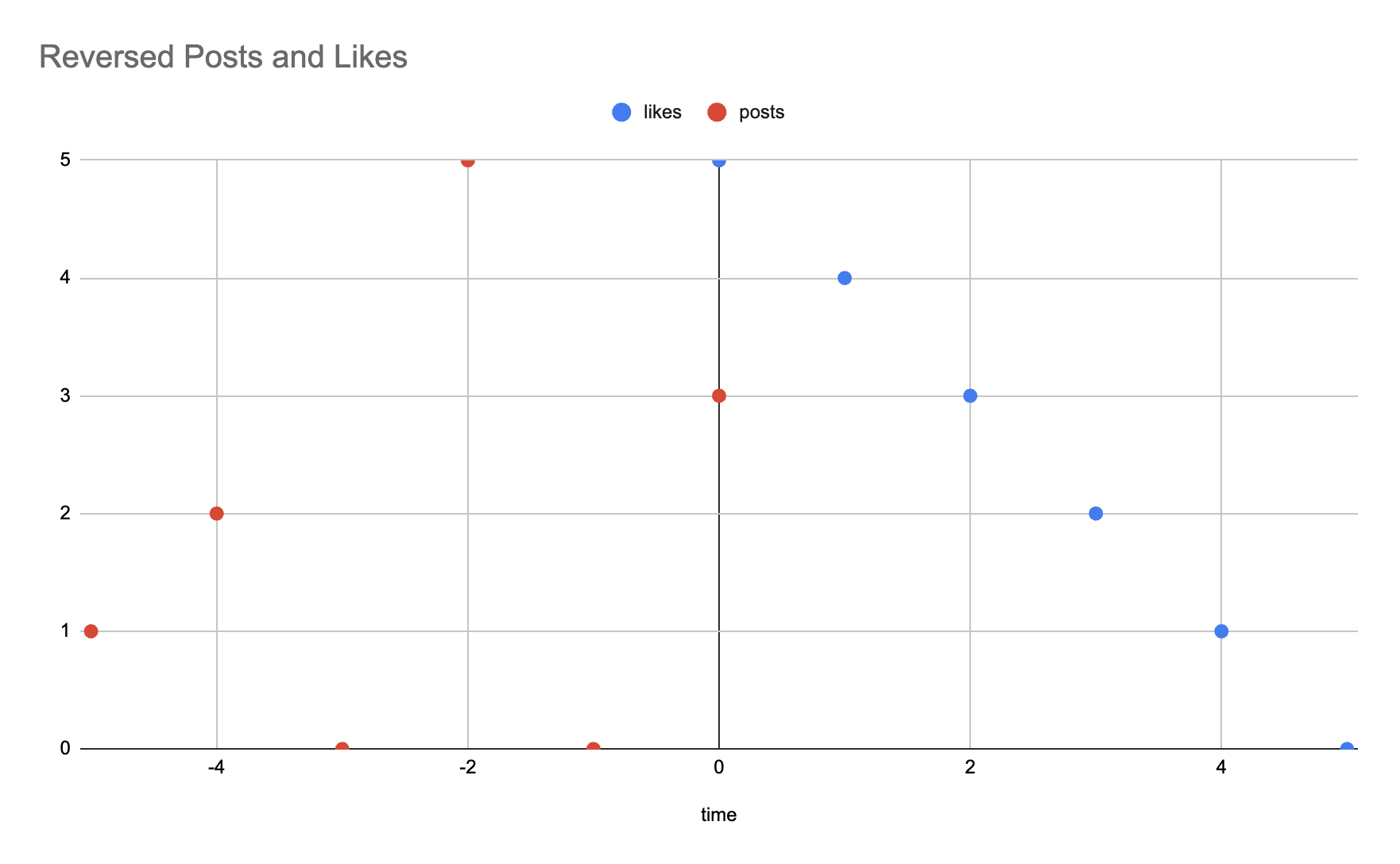
Returning to simplified from the previous section, let’s flip the graph of published posts over time across the y-axis. At $t=0$, 3 is given as the input and the expected likes per each post is 5. Therefore, 15 is the total likes collected at $t=0$.

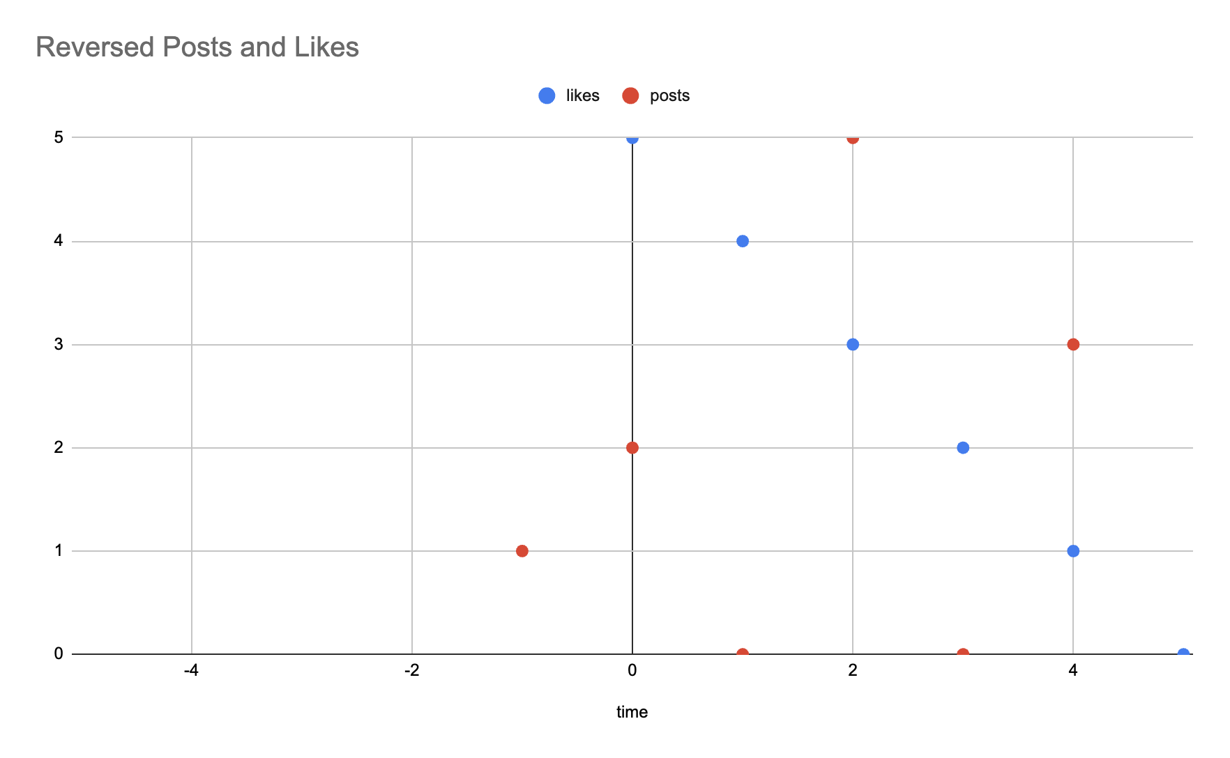
At $t=4$, we can compute:

$ (3 * 1) + (5 * 3) + (5 * 2) = 28 $

And you can verify that the computed output at $t=0$ and $t=4$ match with the ones from the previous section.

Tabluar Example

We can also derive the equation using the tabular form for discrete case. Using the convolution equation in discrete-time:

\[(x * h)[n] = \sum_{m=-\infty}^{\infty} x[m]\,h[n-m],\; m \in \mathbb{Z}.\]

time	0	1	2	⋯	n
x[0]	x[0]h[0]	x[0]h[1]	x[0]h[2]	⋯	x[0]h[n]
x[1]	0	x[1]h[0]	x[1]h[1]	⋯	x[1]h[n-1]
x[2]	0	0	x[2]h[0]	⋯	x[2]h[n-2]
⋮	⋮	⋮	⋮	⋯	⋮
x[m]	0	0	0	⋯	x[m]h[n-m]

Each row of the array is just a scaled, time‑shifted copy of the impulse response, and together these rows sum to form the overall output $y$ for the input signal $x$. To find the output at a particular instant $n$, simply look at the $n$-th column and add its entries—their sum gives $y(n)$:

\[y[n] = x[0]h[n] + x[1]h[n-1] + x[2]h[n-2] + ⋯ + x[m]h[n-m]\]

Conclusion

Convolution is a powerful mathematical operation that combines two functions to produce a third function, capturing how one function modifies the other. Through our exploration, we’ve seen how convolution:

• Preserves temporal relationships in signals
• Handles continuous and discrete time domains
• Provides a framework for analyzing system responses
• Offers intuitive understanding through practical examples

This understanding of convolution forms the foundation for Convolutional Neural Networks (CNNs), where the same principles are applied to process visual data. In CNNs, convolution operations will be used to:

• Detect features in images through learned filters
• Preserve spatial relationships in the data
• Build hierarchical representations of visual information

While this post focused on the mathematical foundations of convolution, these concepts will be essential as we explore how CNNs leverage convolution to achieve remarkable success in computer vision tasks.

Resources

• Convolution in the time domain
• Signal Processing: Flipping the Impulse Response in Convolution
• Intuitive Understanding of Convolution