Efficient Inference Engine on Compressed Deep Neural Network

EIE: Efficient Inference Engine on Compressed Deep Neural Network

Terminology

• DRAM: Dynamic Random-Access Memory, used for large off-chip storage but consumes high energy per access. EIE avoids DRAM by keeping compressed models in on-chip memory.

• SRAM: Static Random-Access Memory, fast and energy-efficient on-chip memory used in EIE to store weights, activations, and intermediate data.

• Processing Element: A lightweight compute core in EIE responsible for storing a partition of the weight matrix and performing multiply-accumulate operations for non-zero activations.

• Dynamic Sparsity: The runtime sparsity in the input activation vector, typically introduced by functions like ReLU. EIE exploits this by skipping computation for zero activations.

• Static Sparsity: The sparsity in the weight matrix resulting from pruning during or after training. These zeros are fixed and encoded in compressed storage formats.

• Weight Sharing: A technique where multiple weights share the same value, represented by a small index into a shared codebook. EIE uses 4-bit weight sharing to reduce memory and computation cost.

Abstract

• Modern state-of-the-art deep neural networks have hundreds of millions parameters which induce expensive computation and memory bandwidth.
• Such increase in the model size and computational capacity make deployment on embedded systems with limited hardware resources especially difficult.
• This paper proposes Efficient Inference Engine (EIE) which:
  • Performs inference on compressed network model (e.g., pruning & quantization)
  • Accelerates the resulting matrix-vector multiplication with weight sharing
  • Performs the operation on SRAM instead of DRAM which saves the energy (measured pJ) by 120x

Introduction & Motivation

• Neural Networks have become ubiquitous in applications including computer vision, speech recognition, and natural language processing. And connections are becoming deeper and more complex:
  • LeNet (1998) handwritten digits classifier: 1M
  • Krizhevsky ImageNet (2012): 60M
  • Deepface Human Face Verification (2014): 120M
• Large DNN are very powerful but consume large amounts of energy because the model must be stored in external DRAM, and fetched every time for each image, word, or speech sample.

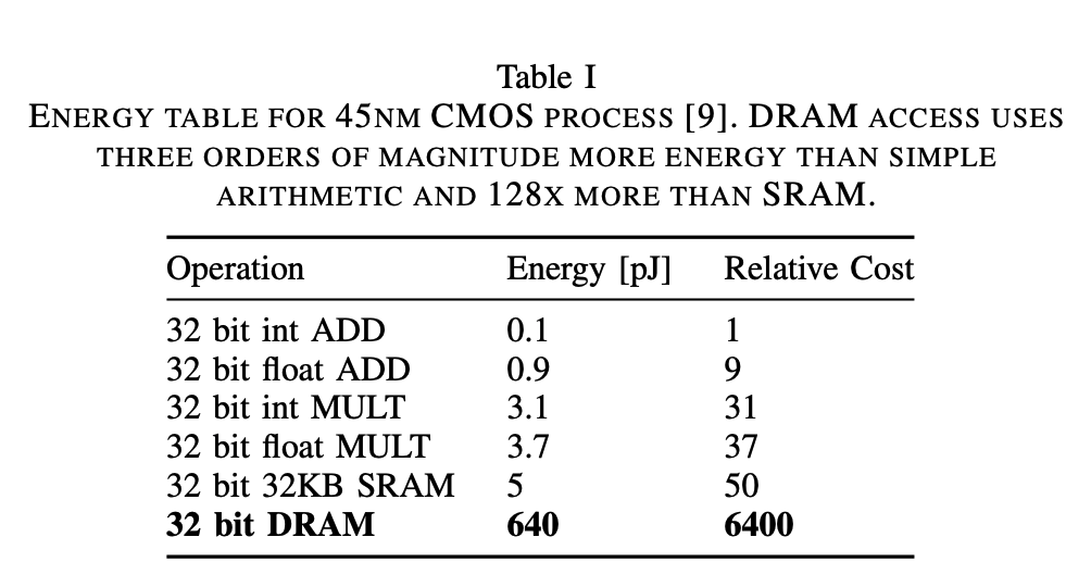
• As shown in the table, total energy is dominated by the memory access. The energy cost per fetch ranges from 5pJ in on-chip SRAM to 60pJ for off-chip DRAM.
• DRAM access requires higher energy consumption which is well beyond the power envelope of a typical mobile device.
• Previous works specialize in accelerating dense and uncompressed neural networks which pose problems in:
  • Limited utility to small models
  • Limited to cases where the DRAM access is tolerable
• Efficient processing of data is also heavily reliant on the model architecture:
  • Convolutional Neural Network (CNN)
    • Data reuse and manipulation is quite suitable for customized hardware. For example, the kernel (filter) weights are reused over many positions in the input.
    • Such reusability of weights make CNN relatively hardware friendly than Fully-Connected layers especially for caches and on-chip SRAM.
  • Fully-Connected (FC) Layers
    • Every output neuron is tightly connected to every input - there’s no reuse of weights across multiple inputs.
    • In large networks, the weight matrix is huge and must be loaded fresh for every input.
    • Such reliability leads to high DRAM bandwidth demand making it inefficient on hardware.
    • Batch: Sharing weights and biases in a batch tolerates SRAM access, however, this is limited to training phase which latency is not a problem.
• Network compression via pruning and weight sharing allows fitting modern networks (e.g., AlexNet, VGG-16) in on-chip SRAM. However, compressed networks raise problems such as:
  • Data Sparsity: With pruning, matrix becomes sparse due to increased zero elements in the matrix.
  • Data Indirection: Non-zero elements are stored in relative indices which adds extra levels of indirection that cause complexity and inefficiency on CPUs and GPUs.

Efficient Inference Engine (EIE)

• This paper proposes EIE, an efficient inference engines, a specialized accelerator that performs customized sparse matrix vector multiplication and handles weight sharing with no loss of efficiency.
  • EIE uses Processing Elements (PEs), each responsible for storing a portion of the neural network in SRAM and performing the parallel computations for that segment. By distributing the network across an array of PEs, EIE efficiently exploits several key optimizations:
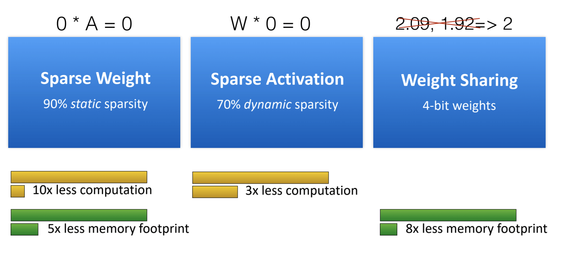
    • Dynamic Sparsity in the input vector
    • Static Sparsity in the weights
    • Relative Indexing for compact storage
    • Weight Sharing to reduce redundancy
    • Extreme narrow weight representations to minimize memory and computation costs

Computation

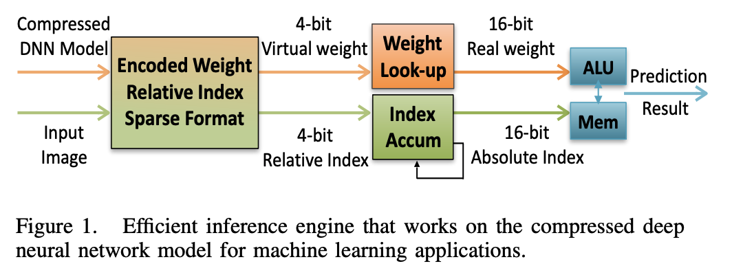
Let’s go through a simplified example for the diagram below which applies matrix-vector multiplication using encoding and weight look-up.

A FC layer of a DNN performs the computation: \(b = f(Wa + v)\)

Where:

• $a$: input activation vector
• $b$: output activation vector
• $v$: bias
• $f$: non-linear activation function

In EIE, pre-activation computation of deep compressed DNN becomes:

\[b_i = \text{ReLU} \left( \sum_{j \in X_i \cap Y} S[I_{ij}] \cdot a_j \right)\]

Where:

• $X_i$: Set of columns $j$ for which $W_{ij} \neq 0$
• $Y$: Set of indices $j$ for which $a_{ij} \neq 0$
• $S$: Table of shared weights (i.e., codebook)
• $I_{ij}$: Index of the shared weight that replaces $W_{ij}$

Dynamic and Static Sparsity

As mentioned in the terminology section, we should be aware of dynamic and static sparsity of the pruned network. From the mathematical expression above:

• $X_i$ represents the static sparsity of $W$
• $Y$ represents the dynamic sparsity of $a$

Example

We will go through an example to understand how EIE uses below to encode and handle matrix-vector multiplication:

• Weight Sharing
• Relative Indexing
• Weight Look up

Suppose we are computing:

\[y = W \cdot x^\top\]

Given:

• $W \in \mathbb{R}^{4 \times 5}$: Weight
• $x \in \mathbb{R}^{1 \times 5}$: Input
• $Y \in \mathbb{R}^{4 \times 1}$: Output

Let’s say $W$ is a sparse matrix of

\[W = \begin{bmatrix} 0 & 0 & 0 & 2.1 & 0 \\ 0 & 3.0 & 0 & 0 & 4.1 \\ 1.2 & 0 & 0 & 0 & 0 \\ 0 & 0 & 5.3 & 0 & 0 \end{bmatrix}\]

And input vector $x$ is:

\[x = [1, 0, 0, 2, 0]\]

Weight Sharing via K-means

Using K-means clustering, a method to partition $n$ observations into $k$ clusters in which each observation belongs to the cluster with the nearest mean clauster, we can partition the matrix $W$ into (also remember the weights are now stored in 8-bit instead of 32-bit):

Original	Closest Cluster	Index
2.1	2.0	1
3.0	3.0	2
4.1	4.0	3
1.2	1.0	0
5.3	5.0	4

Apply Relative Indexing

Now, we can encode the column positions using relative indexing starting from prev_col=-1.

Row	Nonzero Columns	Relative Indices	Codebook Indices
0	[3]	[3 - (-1) = 4]	[1]
1	[1, 4]	[1 - (-1) = 2, 4 - 1 = 3]	[2, 3]
2	[0]	[0 - (-1) = 1]	[0]
3	[2]	[2 - (-1) = 3]	[4]

Perform Sparse Matrix-Vector Multiplication

Compute $y = W \cdot x^\top$ using the compressed format

• Row 0: (rel=4, idx=1)
  • prev_col + rel_col = -1 + 4 = 3
  • x[3] * codebook[1] = 2 * 2 = 4.0
  • y[0] = 4.0
• Row 1: (rel=2, idx=2) & (rel=3, idx=3)
  • prev_col + rel_col:
    • -1 + 2 = 1, x[1] = 0, skip
    • 1 + 3 = 4, x[4] = 0, skip
• Row 2: (rel=1, idx=0)
  • prev_col + rel_col = -1 + 1 = 0
  • x[0] * codebook[0] = 1 * 1 = 1.0
  • y[2] = 1.0
• Row 3: (rel=3, idx=4)
  • prev_col + rel_col = -1 + 3 = 2, x[2] = 0, skip

Therfore:

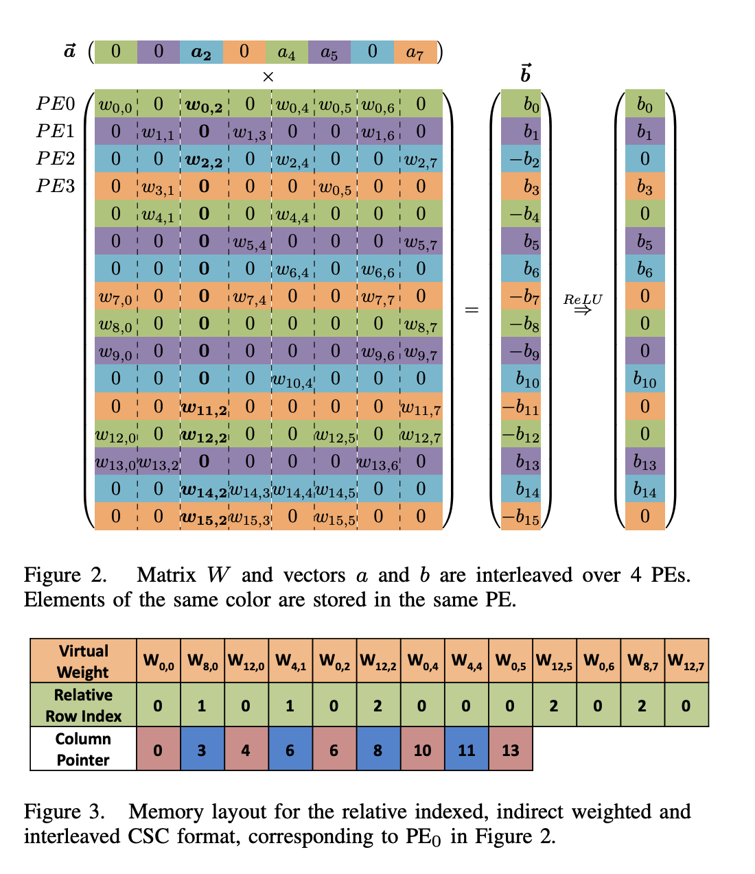
\[y = [4.0, 0.0, 1.0, 0.0]^\top\]

Figure 2 & 3 expand the mathematical concept used in the example above to Processing Elements (PEs) using a Compressed Sparse Columns (CSC)

Architecture & Parallelization

Leading Non-Zero Dectection (LNZD) Node

• Each group of 4 PEs do local LNZD detection
  • The full sparse input vector $a$ is partitioned across the PEs
  • Each PE stores only a chunk of the original input vector in its local SRAM
  • EIE processes one non-zero a_j at a time
• Local LNZD detections done by the PEs are sent to the LNZD Node
  • The LNZD Node will send the result upto the Central Control Unit (CCU) (i.e., the root of LNZD node)
• The CCU will broadcast the selected non-zero activation’s index & value back to each PE using separate wires place in the H-tree

           CCU
           / \
       Node   Node
       / \     / \
     PE  PE   PE  PE

PE Architecture

Activation Queue (FIFO)

• Handles the non-zero inputs broadcasted by CCU
• Stores each non-zero input activation $a_j$ and its index $j$ as it arrives from CCU
• Uses First-In-First-Out (FIFO) structure to ensure activations are processed in order. FIFO enables:
  • Disable Broadcast: If a PE’s queue is full, the CCU pauses further broadcasts to avoid overflow.
  • Load Balancing: Some PEs may be slower (due to sparsity imbalance), so queuing avoids stalling faster ones.

Pointer Read Unit

When PE receives an input activation, Pointer Read Unit helps PE to answer this question

“I just got $a_j$, where should I look in my compressed matrix for non-zero weights in column $j$?”

• Given the start and end pointer indicating where the weights for that column lives in a compressed memory.
• When a_j arrives, the PE looks up start_ptr[j] and end_ptr[j] to take the rows that have non-zero weights in column $j$.
• Multiply each one by a_j and accumulate into output y_i.

Activation Queue & Pointer Read Unit Combined

1. CCU broadcasts: $a_j$ and index $j$

2. Each PE adds it to its Activation FIFO

3. When the PE is ready:

   • Deqeues $a_j$
   • Uses Pointer Read Unit to find where its relevant weights for column $j$ are stored
   • Looks up the corresponding rows and codebook indices
   • Multiplies and accumulates: $\ y_i \mathrel{+}= W_{i, j} \cdot a_j $

Sparse Matrix Read Unit

• Responsible for reading the non-zero weights from the compressed sparse matrix stored inside the PE
  • Takes start and end pointers (from the Pointer Read Unit) for a given column $j$ of $W$
• Reads compressed entries from Sparse Matrix SRAM

Arithmetic Unit

• Responsible of mathematical operation such as:

\[b_x = b_x + v \cdot a_j\]

Where:

• $a_j$: Broadcasted input activation from activatio queue
• $v$: Decoded weight value
• $x$: Output activation index (tells us which row of $y$ this affects)

Activation Read / Write Unit

• Handles how input and output activations are stored and passed between layers efficiently and with minimal data movement
• Each PE has two registers:
  • Reading input activations (source)
    • Holds a slice of the input activation vector $a$ for this layer
  • Writing output activations (destination)
    • Holds a slice of the output activation vector $b$ for the next layer
• After computing one layer, the role swaps:
  • Destination becomes the next layer’s source
• This register file role-exchange minimizes unnecessary data transfers, which saves energy and bandwidth

Conclusion

EIE is a custom hardware accelerator designed for compressed deep neural networks, especially for fully-connected (FC) layers.

It achieves massive energe savings (up to 3,400× vs GPU) by leveraging:

• 10× weight pruning
• 4-bit weight sharing (quantization)
• On-chip SRAM storage instead of DRAM (120× energy saving)
• Dynamic activation sparsity (only ~30% of matrix columns accessed)

Performance Gains on 9 FC-layer Benchmarks:

• 189× faster than CPU
• 13× faster than GPU
• 307× faster than mobile GPU

Energy Efficiency Gains:

• 24,000× less energy than CPU
• 3,400× less energy than GPU
• 2,700× less energy than mobile GPU

Resources

• EIE: Efficient Inference Engine on Compressed Deep Neural Network
• Efficient Inference Engine on Compressed Deep Neural Network
• Efficient Inference Engine on Compressed Deep Neural Network