Linearity and Linear Transformation
Introduction
In our previous post, we explored the fundamental concept of derivatives and their application in neural networks. We manually performed backpropagation using the chain rule, adjusting the parameters (specifically, the leaf nodes) to refine the output through incremental updates.
Before diving deeper into the construction of more complex neural networks, we will take some time to explore the concepts of vectors, matrices, and linear transformations. These are essential foundations because, at its core, a neural network is an insane matrix multiplications machine that scales and transforms the inputs.
Problem Statement: XOR Gate

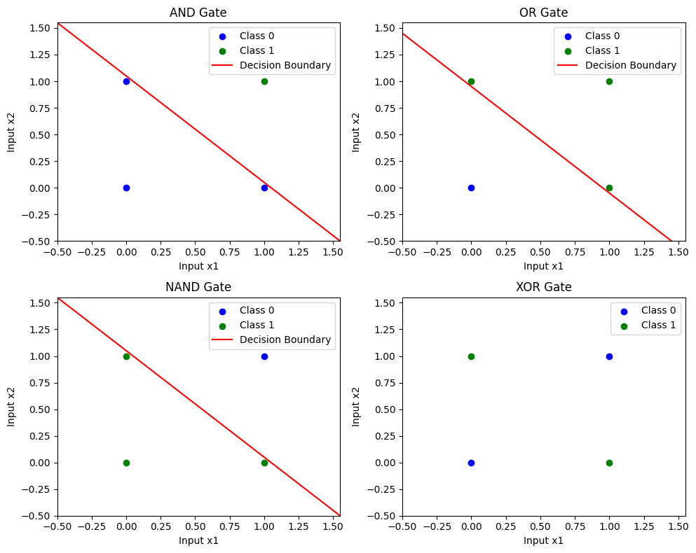
The XOR Gate(exclusive OR) problem is a logical gate that outputs True only when the inputs differ (i.e., one is true and the other is false). In contrast to logical gates like AND, OR, and NAND, which are linearly separable in 2D space (meaning their decision boundaries can be represented by a straight line that divides points of different classes), the XOR gate cannot be separated linearly in a 2D space.
This seemingly simple challenge led to confusion among early artificial neural network (ANN) researchers and was one of the key reasons behind the AI Winter of the 1970s. The breakthrough solution to the XOR problem came with the introduction of Multi-Layer Perceptron (MLP) networks that contain at least one hidden layer, coupled with non-linear activation functions.
A crucial insight in solving this problem is the idea of projecting the input space into a higher dimension. By transforming the original 2D space into a higher-dimensional space, the XOR points that were previously inseparable can become linearly separable. This transformation allows the network to draw a decision boundary that correctly classifies the inputs, thus making it possible for MLPs to solve the XOR problem.
The Value class, as implemented in previous post, forms the foundation for constructing a simple neural network. However, there are two key limitations with the current setup:
- Scalar Computations Only: The class is designed for scalar operations like addition and multiplication, whereas a typical MLP performs operations involving multiple weights and biases simultaneously (vectorized or matrix computations).
- No Non-Linear Activation Functions: The current implementation lacks non-linear activation functions, which are essential in MLPs to introduce the non-linear decision boundaries needed for solving problems like XOR or enabling the network to approximate complex functions.
Quick Review on Vector
The concept of a vector carries different nuances across fields like Physics, Computer Science, and Mathematics. For simplicity in this post, we will rely on the mathematical definition:
A vector is an abstract object in a vector space, which satisfies certain axioms like addition and scalar multiplication.
Using the concept of a vector space to define a vector might feel a bit circular, but it is a practical approach. This definition emphasizes that any objects meeting these conditions can be considered and utilized as vectors.
Vector Addition: \(\mathbf{V} \neq \emptyset, \; \mathbf{a}, \mathbf{b} \in \mathbf{V} \implies \mathbf{a} + \mathbf{b} \in \mathbf{V}\)
Scalar Multiplication: \(\mathbf{V} \neq \emptyset, \; \mathbf{a} \in \mathbf{V}, \; \mathbf{c} \in \mathbb{R} \implies \mathbf{c} \cdot \mathbf{a} \in \mathbf{V}\)
Using the axioms above, we can express linear combination of two vectors that maps to entire vectors in 2-dimensional space (or in other words a span):
\[\mathbf{c1}, \mathbf{c2} \in \mathbb{R} \implies \mathbf{c1} \cdot \begin{bmatrix} 1 \\ 0 \end{bmatrix} + \mathbf{c2} \cdot \begin{bmatrix} 0 \\ 1 \end{bmatrix} \in \mathbb{R^2}\]Implication of Matrix Multiplication
The vector definition that we set above gives new interpretation of matrix-vector multiplication. Given a matrix-vector multiplication form of:
\[\begin{bmatrix} a & b \\ c & d \end{bmatrix} \begin{bmatrix} x \\ y \end{bmatrix} = \begin{bmatrix} ax + by \\ cd + dy \end{bmatrix}\]We can also re-write this as:
\[\begin{bmatrix} a & b \\ c & d \end{bmatrix} \begin{bmatrix} x \\ y \end{bmatrix} = x \cdot \begin{bmatrix} a \\ c \end{bmatrix} + y \cdot \begin{bmatrix} b \\ d \end{bmatrix}\]Matrix-vector multiplication represents the linear combination of the column vectors of the matrix, weighted by the corresponding elements of the vector. This operation generates a new vector within the vector space spanned by the matrix’s column vectors.
In other words, the multiplication highlights the potential to create vectors within the span (vector space) defined by the column vectors of the matrix. Thus, the result of the matrix-vector multiplication lies in the subspace formed by these column vectors.
Although, we have not fully covered the neurons, multilayer perceptrons and forward pass of MLP, try to make familiarize to the expression below:
\[\vec{y} = W\vec{X} + \vec{b}\]Where:
- $\vec{y}$: Output Vector (2 x 1)
- $W$: Weight Matrix (2 x 2)
- $\vec{X}$: Input Data Vector (2 x 1)
- $\vec{b}$: Bias Vector (2 x 1)
Let’s assign random values to $W$, $\vec{X}$ and $\vec{b}$:
\[\begin{aligned} W &= \begin{bmatrix} 1 & 2 \\ 3 & 4 \end{bmatrix}, \quad \vec{X} = \begin{bmatrix} a \\ b \end{bmatrix}, \quad \vec{b} = \begin{bmatrix} 5 \\ 6 \end{bmatrix} \end{aligned}\]Therefore:
\[\vec{y} = W\vec{X} + \vec{b} = \begin{bmatrix} 1 & 2 \\ 3 & 4 \end{bmatrix} \cdot \begin{bmatrix} a \\ b \end{bmatrix} + \begin{bmatrix} 5 \\ 6 \end{bmatrix} = \begin{bmatrix} a + 2b + 5 \\ 3a + 4b + 6 \end{bmatrix}\]With this expression in my mind, we can ask:
- Does $y$ exist in the vector space created by column vectors $\begin{bmatrix} 1 \ 3 \end{bmatrix}$, $\begin{bmatrix} 2 \ 4 \end{bmatrix}$ and $\begin{bmatrix} 5 \ 6 \end{bmatrix}$?
- If so, how should we linearly transform those column vectors to create $y$?
Linear Transformation
We’ve taken quite a detour to arrive at today’s topic — linear transformation. However, the journey has been worthwhile, as it has prepared us to understand how an input vector is transformed into a new output vector, mapped to a different vector space through matrix multiplication.
This brings us to another interpretation of matrix-vector multiplication: the matrix acts as a function that accepts a vector as input and outputs a transformed vector:
\[\begin{bmatrix} a & b \\ c & d \end{bmatrix} \left( \begin{bmatrix} x \\ y \end{bmatrix} \right)\]In linear algebra, the term transformation is often used interchangeably with function. So, why not use linear function instead of linear transformation? The term transformation is preferred because it emphasizes the process of mapping or moving vectors between spaces, underscoring the geometric aspect of the operation.
If a transformation, $T$ on set of vectors $v_1, v_2, …, v_n$ and scalars $c_1, c_2, …, c_n$ satifies conditions below, $T$ is a linear combination:
- Additivity: \(T(u + v) = T(u) + T(v)\)
- Homogenity: \(T(cv) = c \cdot T(v)\)
Using these axioms, we can deduce where any vectors will land so long as we know where the basis vectors which compose the vector space will land.
Given two basis vectors $i$ and $j$:
\[\begin{aligned} i &= \begin{bmatrix} 1 \\ 0 \end{bmatrix}, \quad j = \begin{bmatrix} 0 \\ 1 \end{bmatrix} \end{aligned}\]Let’s say $i$ and $j$ are transformed into new vectors $\hat{i}$ and $\hat{j}$ respectively by:
\[\begin{aligned} \hat{i} = T(i), \quad \hat{j} = T(j) \end{aligned}\]Then a $\vec{v}$ of $[x, y]^T$:
\[T\left( \begin{bmatrix} x \\ y \end{bmatrix} \right) = x \cdot T(i) + y \cdot T(j) = x \cdot \hat{i} + y \cdot \hat{j}\]Therefore, a 2D linear transformation of $\vec{v}$ can be described using a matrix of of 4 numbers which stores the coordinates of $\hat{i}$ and $\hat{j}$ (so long as the basis vectors $i$ and $j$ are linearly independent).
Non-linearity & Activation Function
Let’s now go back to the XOR problem that we discussed earlier. Two major approaches to enable simple perceptrons to solve the XOR problem are:
- Multi-layer Perceptrons (MLPs): By introducing additional hidden layers, the network can learn intermediary features and construct complex non-linear decision boundaries.
-
Activation Functions: These introduce non-linearity by applying functions such as
sigmoid,tanh, orReLUto the linear transformations. This allows the network to capture the non-linear relationship between inputs and outputs. In the case of XOR, the labels are not linearly separable in a two-dimensional space.
And this is where the concept of linear combination that we have covered so far and non-linearity of activation functions should start to click.
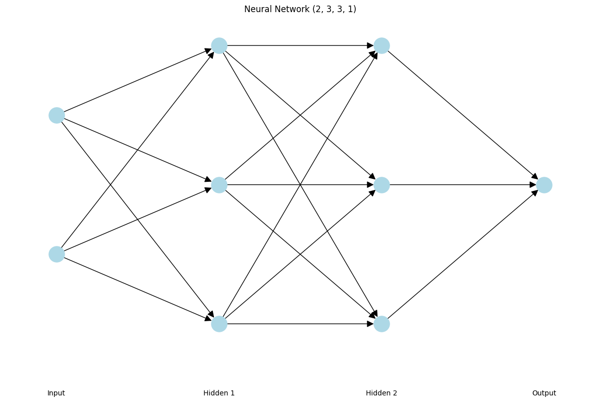
Let’s say we have a MLP with structure of (2, 3, 3, 1):

- Input: 2 neurons
- Hidden Layers: 2 hidden layers with 3 neurons each
- Output: 1 neuron
Each layer’s output is computed as a linear transformation of (recall this is exactly identical to the $\vec{y} = W\vec{X} + \vec{b}$ from above):
\[z^l = W^l \cdot z^{l-1} + b^l\]Where:
- $W^l$: Weight matrix of layer $l$
- $z^{l-1}$: Linear transformation (output) of the previous layer
- $b^l$: Bias vector of layer $l$
If there is no activation function in the network, output $z^l$ remains a linear transformation of the input:
\[\begin{aligned} z^1 &= W^1 \cdot X + b^1 \\ z^2 &= W^2 \cdot z^1 + b^2 \\ z^3 &= W^3 \cdot z^2 + b^3 \\ z^3 &= W^3 \cdot (W^2 \cdot (W^1 \cdot X + b^1) + b^2) + b^3 \end{aligned}\]Which simplies to:
\[z^3 = \tilde{W} \cdot X + \tilde{b}\]Where:
- $\tilde{W} = W^3 \cdot W^2 \cdot W^1$: Effective weight matrix combining all transformations.
- $\tilde{b}$: Effective bias vector.
Conclusion
We began by exploring the fundamental operations of vectors, understanding matrix-vector multiplication, and examining various interpretations of linear transformations. We then discussed how a neural network without a non-linear activation function is simply a stack of linear transformations, rendering it ineffective for solving non-linear problems.
As mentioned earlier, there are many activation functions, each with unique attributes and limitations, which we will delve into in a future post.
Having established the importance of introducing non-linearity, we are now well-equipped to design a complex multi-layer perceptron with activation functions.