Negative Log Likelihood Explained

Introduction

In our previous post, we explored a bigram language model that predicts the next character in a sequence based on probability distributions. At the heart of this model was the negative log likelihood loss function, which helped us evaluate and optimize its performance. When training a neural network, understanding the loss function is crucial for evaluating the model’s performance and optimizing its parameters.

This post will provide a solid understanding of the fundamental concepts: probability, likelihood, log likelihood, maximum likelihood estimation, and negative log likelihood.

Probability vs. Likelihood

Q: “How likely is it that the coin will land heads?”
A: “Probable if you’re talking about the event, likely if you’re fitting parameters to data!”

— Overheard at a Statistician's bar

In statistics, the term probability and likelihood can not be used interchangeably, and hold different implications. Understanding the subtle difference between the two is crucial for understanding the concept of maximum likelihood estimation.

Probability

Probability measures how likely an event (x) is to occur given fixed parameters (θ). In other words, it answers the question: “Given these parameters, what’s the chance of seeing this data?”

Mathematically, we express this as:

\[P(x \mid \theta)\]

Where:

• $x$: the observed data (event)
• $\theta$: the fixed parameters
• $P(x \mid \theta)$: the probability of $x$ given $\theta$

Probability Diagram Explained

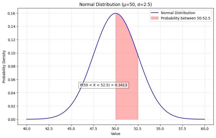
The diagram above illustrates a normal distribution with mean (μ) = 50.0 and standard deviation (σ) = 2.5. The shaded area represents the probability of observing a value between 50.0 and 52.5, which equals 0.3413 (or about 34.13%). This can be understood using the empirical rule (also known as the 68-95-99.7 rule) for normal distributions:

• 68% of the data falls within μ ± 1σ (47.5 to 52.5)
• 95% of the data falls within μ ± 2σ (45.0 to 55.0)
• 99.7% of the data falls within μ ± 3σ (42.5 to 57.5)

In this case, the area we’re measuring (50.0 to 52.5) represents exactly half of the 68% region above the mean, hence 0.68/2 ≈ 0.3413.

Likelihood

Likelihood measures how well parameters (θ) explain observed data (x). In other words, it answers the question: “Given this observed data, how good are these parameters at explaining it?”

Mathematically, we express this as:

\[L(\theta \mid x)\]

Where:

• $\theta$: the parameters to be estimated
• $x$: the fixed observed data
• $L(\theta \mid x)$: the likelihood of parameters $\theta$ given the observed data $x$

Likelihood Diagram Explained

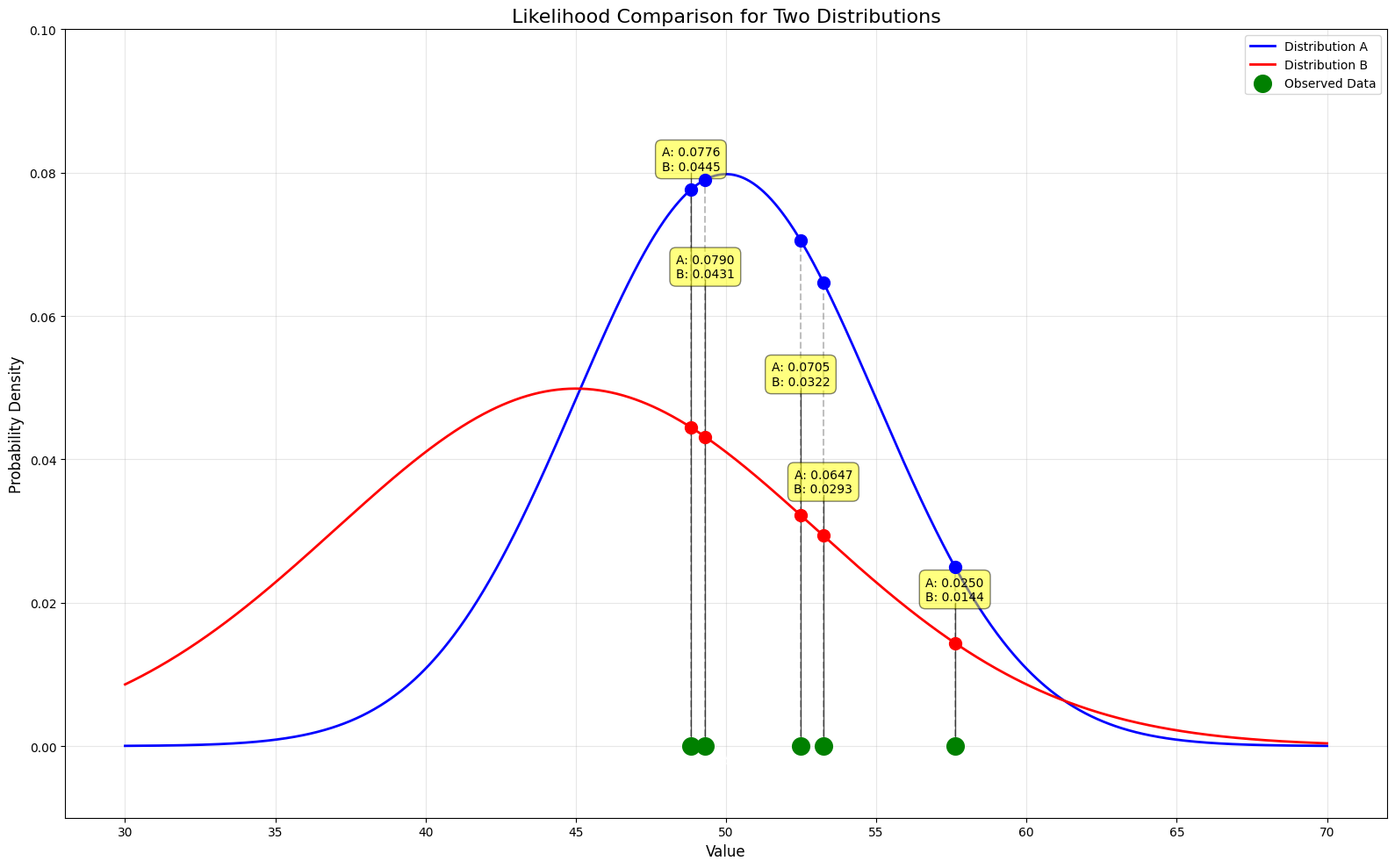
data = [48.8292 49.3087 52.4836 53.2384 57.6151]
likelihood_A = [0.0776, 0.0790, 0.0705, 0.0647, 0.0250]
likelihood_B = [0.0445, 0.0431, 0.0322, 0.0293, 0.0144]

The diagram above shows a 5-data points from a normal distribution with mean (μ) = 52.295 and standard deviation (σ) = 3.167.

Just glancing at the diagram, we can see that the likelihood of observing these data points is higher for Distribution A than Distribution B:

• The distribution of observed data points is more concentrated around the mean of Distribution A than Distribution B.
• The likelihood of observing these data points is higher for Distribution A than Distribution B.

The likelihood of observing these data points is calculated by multiplying the probability of each data point given the parameters. Therefore the likelihood of observing these data in each distribution is (make sure to remember how the probability is extremely small as a result of the multiplication):

• Distribution A: 6.99072501e-07 or 0.000000699072501
• Distribution B: 2.6056931140799998e-08 or 0.000000026056931140799998

Likelihood Function

Based on the example above, we realize that by observing the data, we can estimate the parameters of the distribution. And likelihood simply measures how “likely” the observed data is from the distribution.

A mathematical representation of the likelihood function is:

\[L(\theta \mid x) = \prod_{i=1}^{n} P(x_i \mid \theta)\]

Log Likelihood

Log likelihood is the logarithm of the likelihood function, expressed as:

\[\log L(\theta \mid x) = \sum_{i=1}^{n} \log P(x_i \mid \theta)\]

If you need a quick refresher on logarithm, I recommend watching 3b1b’s lecture.

Log likelihood is a more convenient function to work with because of:

• Numerical Stability: Probabilities can be very small, and products of probabilities will be much smaller. Such small probabilities can lead to numerical underflow in computers.
• Simplified Computation: Logarithms transform products into sums, which are easier to handle mathematically.
• Identical Maximizer: The maximum likelihood estimate is the same for both the likelihood and log-likelihood functions.

Example: Log Likelihood

This example demonstrates how logarithms make likelihood calculations more manageable:

1. The raw likelihood calculation (0.015 * 0.05 * 0.01) results in a tiny number (7.5e-06) that is hard to work with computationally.

2. By using logarithms, we:

   • Convert multiplications to additions: log(a * b * c) = log(a) + log(b) + log(c)
   • Transform tiny numbers into more manageable negative values: 7.5e-06 → -11.80

This simple transformation makes calculations numerically stable and computationally efficient.

"""
log(a * b * c) = log(a) + log(b) + log(c)
"""
import torch

# Likelihood values
likelihood_A = 0.015
likelihood_B = 0.05
likelihood_C = 0.01

# Likelihood values
total_likelihood = likelihood_A * likelihood_B * likelihood_C

# Log Likelihood values
log_likelihood_A = torch.log(torch.tensor(likelihood_A))
log_likelihood_B = torch.log(torch.tensor(likelihood_B))
log_likelihood_C = torch.log(torch.tensor(likelihood_C))

# Total Log Likelihood
total_log_likelihood = log_likelihood_A + log_likelihood_B + log_likelihood_C

print(f"Total Likelihood: {total_likelihood}")
print(f"Total Log Likelihood: {total_log_likelihood}")

log_applied = torch.log(torch.tensor(total_likelihood))

print(f"Is equal: {log_applied == total_log_likelihood}")

Total Likelihood: 7.5e-06
Total Log Likelihood: -11.800607681274414
Is equal: True

Maximum Likelihood Estimation

Maximum Likelihood Estimation (MLE) is a method for estimating the parameters of a probability distribution by maximizing the likelihood function. In other words, it finds the parameters that make the observed data most probable.

\[\hat{\theta} = \underset{\theta}{\operatorname{argmax}} \, L(\theta \mid x)\]

Where:

• $\hat{\theta}$: the maximum likelihood estimate
• $\theta$: the parameters we’re trying to estimate
• $x$: the observed data
• $L(\theta \mid x)$: the likelihood function

As covered in the previous section, we normally find the maximum of log likelihood function. The maximum can be found by taking the derivative of the log likelihood function with respect to the parameters and setting it to zero.

\[\frac{\partial}{\partial \theta} \log L(\theta \mid x) = \frac{\partial}{\partial \theta} \log P(x \mid \theta) = \sum_{i=1}^{n} \frac{\partial}{\partial \theta} \log P(x_i \mid \theta) = 0\]

If you are interested in the mathematical derivation of the MLE, here are some resources:

• Maximum Likelihood Estimation(MLE): A more complex example of Maximum Likelihood Estimation
• Maximum Likelihood For the Normal Distribution, step-by-step!!!

Negative Log Likelihood

Negative log likelihood is the negative of the log likelihood function, expressed as:

\[- \log L(\theta \mid x) = - \sum_{i=1}^{n} \log P(x_i \mid \theta)\]

It is simply an inverted version of the log likelihood function. Then why use negative log likelihood?

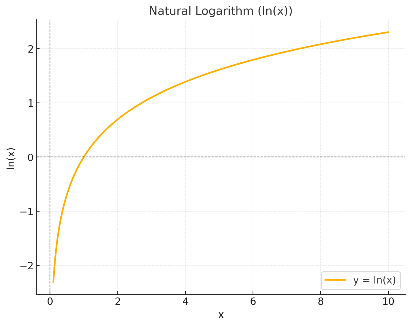
Looking at natural log graph above, let’s think about the upper and lower bound of the function. Since we are assigning probability to the data, the maximum we can get is 1. Therefore, the maximum of the log likelihood is 0. And the lower the probability, the lower the bound of the function (−∞).

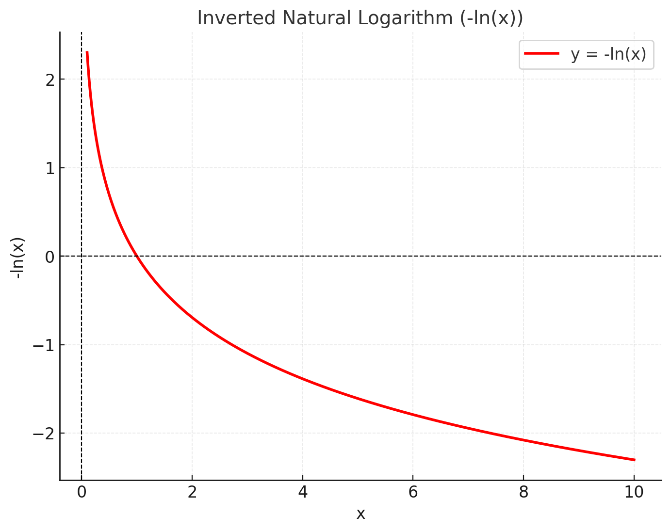
Recalling the optimization steps so far from the previous post, we have tried to find the minimum of the loss function. Therefore, we can use negative log likelihood to transform the task into a minimization problem. Now, when the model assigns probability to the data, the higher the probability, the lower the bound of the function, and vice versa.

This is advantageous because:

1. Optimization Convention: Most optimization algorithms are designed to minimize rather than maximize functions.
2. Gradient Descent: Deep learning frameworks typically implement gradient descent.
3. Loss Function Consistency: Other loss functions (MSE, MAE) are also minimized, making NLL consistent with the broader optimization landscape.

Example

Now, let’s take a look at the code from the previous post and see if concepts we have covered so far were applied correctly.

Steps

1. Convert the log-likelihood to negative log-likelihood
2. Derive the negative log-likelihood with respect to the parameters
3. Update the parameters using gradient descent

# gradient descent
for k in range(1000):
  # forward pass
  xenc = F.one_hot(xs, num_classes=27).float() 
  logits = xenc @ W 
  counts = logits.exp() 
  probs = counts / counts.sum(1, keepdims=True) 
  loss = -probs[torch.arange(num), ys].log().mean() + 0.01*(W**2).mean() # 1. Negative Log Likelihood Conversion
  print(loss.item())
  
  # backward pass
  W.grad = None 
  loss.backward() # 2. Derivation of NLL with respect to W
  
  # update
  W.data += -50 * W.grad # 3. Gradient Descent

Conclusion

In this post, we have covered the concepts of probability, likelihood, log likelihood, maximum likelihood estimation, and negative log likelihood. We have also seen how these concepts are applied in the context of training a neural network.

Training a neural network is essentially finding the parameters that best explain the observed data. And in order to best explain the observed data, we need to maximize the likelihood of the observed data. However, since the loss function in neural network frameworks is a minimization problem, we need to convert the maximization problem into a minimization problem. We solve this by converting the likelihood function into a negative log likelihood function.

We now have a great foundation to learn more about the loss function and optimization in deep learning, and especially Cross Entropy loss function which we will be covering in the next post.

Resources

• In Statistics, Probability is not Likelihood.
• Logarithm Fundamentals | Ep. 6 Lockdown live math
• Maximum Likelihood Estimation(MLE)
• Maximum Likelihood For the Normal Distribution, step-by-step!!!