Bias-Variance Tradeoff and Regularization
Introduction
Machine learning models aim to discover patterns in data by learning the relationships between inputs and outputs. To measure how well a model performs this task, we calculate the difference between its predictions and the actual values using a loss function.
However, achieving perfect accuracy on the training data is not always desirable. When a model learns the training data too precisely, including its noise and outliers, it fails to generalize well to new, unseen data. This phenomenon is known as overfitting. To combat this issue, we employ various regularization techniques that help the model maintain a balance between fitting the training data and generalizing to new examples.
For example, in our previous post on Building a Bigram Character-Level Language Model, we demonstrated this concept by implementing L2 Regularization:
1

loss = -probs[torch.arange(num), ys].log().mean() + 0.01*(W**2).mean() # L2 Regularization
In this post, we will dive deep into L1 and L2 Regularization techniques and explore the theory behind them.
Underfit, Overfit, and Good Fit
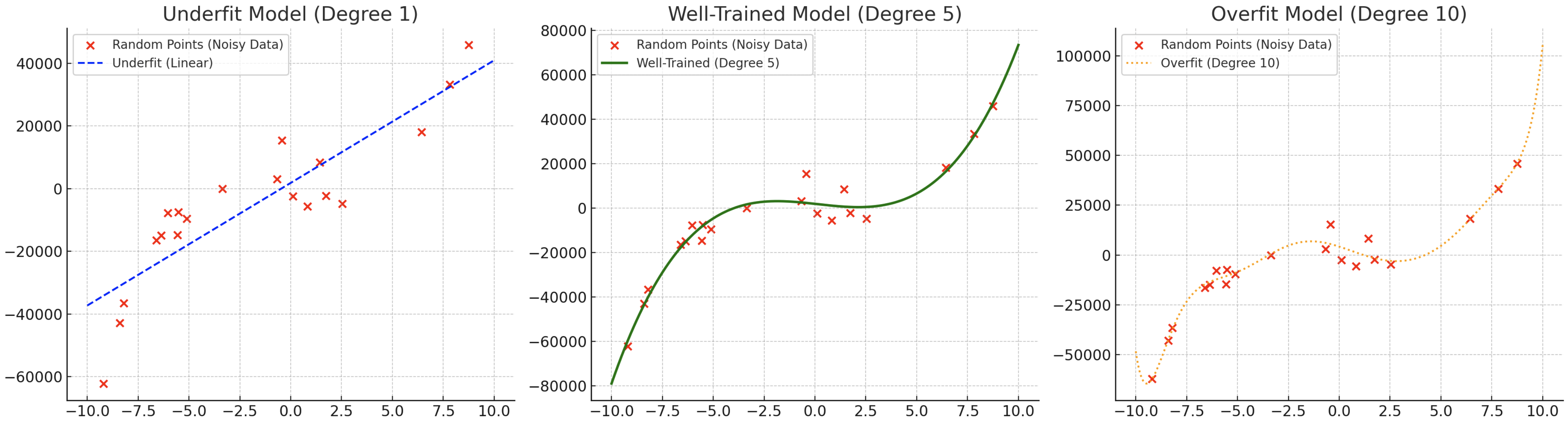
The visualization above demonstrates three different scenarios of model fitting, using data points sampled from the polynomial function ( y = x^5 + 3x + 4 ). Each curve represents a different modeling approach:
Underfitting (High Bias): The linear model (blue line) is too simplistic and fails to capture the polynomial nature of the data. It makes strong assumptions about the relationship being linear, resulting in poor performance on both training and test data.
Good Fit (Balanced): This model (green line) strikes an optimal balance between complexity and simplicity. It successfully captures the underlying polynomial pattern while avoiding the influence of noise in the training data.
Overfitting (High Variance): The complex model (dotted line) fits the training data too precisely, creating an overly complicated function that follows noise and outliers. While it performs exceptionally well on training data, it will likely fail to generalize to new examples.
Bias & Variance
Sidenotes of “high bias” and “high variance” are included next to the underfitting and overfitting curves, respectively. Let’s first understand what these terms mean, and relate to the performance of the model.
Bias
Bias represents the average difference between the expected value of the model’s predictions and the actual value of the target variable.
\[Bias = E[\hat{f}(x)] - f(x)\]Where:
- $\hat{f}(x)$: the predicted value of the model at $x$
- $E[\hat{f}(x)]$: the average predicted value of the model at $x$ across multiple training datasets
- $f(x)$: the actual value of the target variable
- $E$: represents the expectation (mean) over multiple datasets.
Example
Let’s say we train a model on a fuction of $f(x) = x^2$, and the model predicted below for each training dataset:
| x | f(x) | f̂₁(x) | f̂₂(x) | f̂₃(x) | E[f̂(x)] |
|---|---|---|---|---|---|
| 0 | 0 | 0.1 | -0.1 | 0.2 | 0.0667 |
| 1 | 1 | 0.8 | 1.2 | 0.7 | 0.9 |
| 2 | 4 | 4.2 | 4.1 | 4.3 | 4.2 |
| 3 | 9 | 8.8 | 9.2 | 8.5 | 8.83 |
In order to ignore the magnitude of the bias, we can use the squared bias instead:
\[Bias^2 = \left(E[\hat{f}(x)] - f(x)\right)^2\]Variance
Variance measures the variability of the model’s predictions across different training datasets. In other words, it measures how much the model is robust to different training datasets.
\[Variance = E\left[\left(\hat{f}(x) - E[\hat{f}(x)]\right)^2\right]\]Where:
- $\hat{f}(x)$: the predicted value of the model at $x$
- $E[\hat{f}(x)]$: the average predicted value of the model at $x$ across multiple training datasets
Example
| x | f̂₁(x) | f̂₂(x) | f̂₃(x) | E[f̂(x)] |
|---|---|---|---|---|
| 0 | 0.1 | -0.1 | 0.2 | 0.0667 |
| 1 | 0.8 | 1.2 | 0.7 | 0.9 |
| 2 | 4.2 | 4.1 | 4.3 | 4.2 |
| 3 | 8.8 | 9.2 | 8.5 | 8.83 |
Bias-Variance Tradeoff
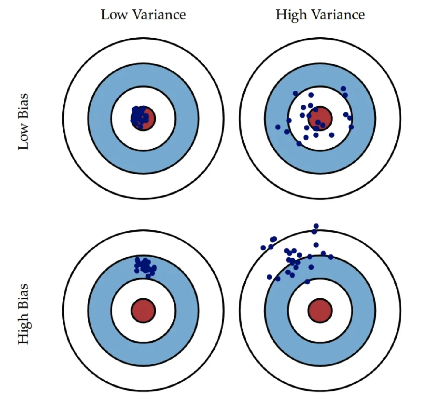
The diagram above categorizes the model’s performance based on the level of bias and variance. The red circle at the center represents the target value which the model is trying to predict.
| Low Variance | High Variance | |
|---|---|---|
| Low Bias | Best Model (Generalizes Well) | Overfitting |
| High Bias | Underfitting | High Bias & High Variance (Worst Case) |
The model with the low bias and low variance is able to predict the most accurate value meanwhile staying robust to the different training datasets.
Once the model is overfitted to the training data, it has learned the noise in the training data as the pattern which performs poorly on the validation and test datasets. In the other hand, if the model if underfitted, it has not fully learned the pattern of the training data which results in poor performance on the training data as well.
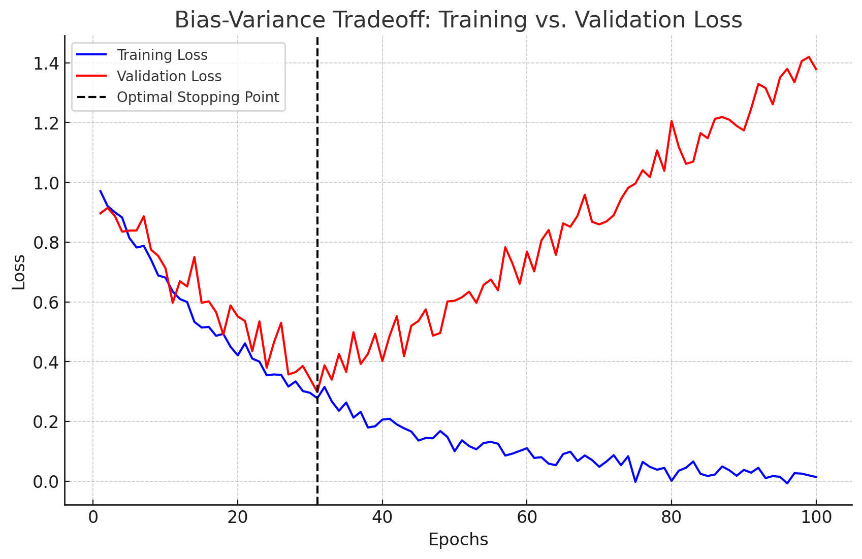
Therefore, the goal of the model is to find the balance between bias and variance to achieve the best performance. It is impossible to lower both the bias and variance at the same time, thus we need to find the optimal point that results in the best performance. The general rule of thumb in this optimal point is to compare the performance of the model on the training data and the validation data.
L1 & L2 Regularization
L1 and L2 regularization are weight decay techniques that prevent overfitting by adding a penalty to the model’s weights. In machine learning, model weights are coefficients that scale input features to make predictions. Larger weights can make the model overly sensitive to small variations in the data, leading to overfitting (memorizing noise rather than generalizing). Regularization reduces large weights, making the model simpler and more robust.
L1 (Lasso) Regularization
Adds a penalty (L1 norm) proportional to the absolute value of the weights.
\[\mathcal{L} = \mathcal{L}_0 + \lambda \sum_{i=1}^n |w_i|\]Where:
- $\mathcal{L}_0$: the loss function of the model
- $\lambda$: the regularization parameter
- $n$: the number of weights
- $w_i$: the $i$-th weight
$\lambda$ is a hyperparameter that controls the strength of the regularization. If $\lambda$ is too large, the model will be too simple and underfit the training data. If $\lambda$ is too small, the regularization will be too weak and the model will overfit the training data.
L1 Regularization tends to shrink some weights to zero, thus creating a sparse model.
L1 Optimization
\[w_{i+1} = w_i - \eta \cdot \frac{dLoss}{dw} = w_i - \eta \left(\frac{\partial \mathcal{L}_0}{\partial w_i} + \lambda \cdot \text{sign}(w_i)\right)\] \[\frac{d}{dw_i}{|w_i|} = \text{sign}(w_i) = \begin{cases} +1, & w_i > 0 \\ -1, & w_i < 0 \\ \text{undefined}, & w_i = 0 \end{cases}\]L1 Optimization Example
Assume we have:
- $w=0.05$
- $\eta=0.1$
- $\frac{dL}{dw}=0.02$
- $\lambda=0.1$
Without regularization,
\[w_{i+1} = w_i - \eta \cdot \frac{dL}{dw} = 0.05 - 0.1 \cdot 0.02 = 0.048\]With regularization,
\[w_{i+1} = w_i - \eta \left(\frac{dL}{dw} + \lambda \cdot \text{sign}(w_i)\right) = 0.05 - 0.1 \cdot \left(0.02 + 0.1 \cdot 1\right) = 0.038\]You can see that the weight shrinks faster compared to the standard gradient descent. And also, the value of $sign{w_i}$ is adding constant value $-1$ or $+1$ multiplied by $\lambda$ to the weight, thus the weight is more likely to be pushed towards zero. In practice, when the weights are close to zero, many optimizers (e.g., Adam, SGD) include a thresholding step:
\[\text{If } |w| < \eta \cdot \lambda, \text{ then set } w = 0\]L2 (Ridge) Regularization
Adds a penalty (L2 norm) proportional to the square of the weights.
\[\mathcal{L} = \mathcal{L}_0 + \lambda \sum_{i=1}^n w_i^2\]L2 Regularization tends to smoothly shrink the weights towards zero, but not to zero.
L2 Optimization
\[w_{i+1} = w_i - \eta \cdot \frac{dLoss}{dw} = w_i - \eta \left(\frac{\partial \mathcal{L}_0}{\partial w_i} + 2\lambda \cdot w_i\right)\]L2 Optimization Example
In this example, we will see how the L2 regularization scales shrinkage with weight magnitude.
Assume we have:
- $w_i=0.05$
- $w_j=0.005$
- $\eta=0.1$
- $\frac{dL}{dw_i}=0.02$
- $\frac{dL}{dw_j}=0.02$
- $\lambda=0.1$
For $w_i$:
\[w_{i+1} = w_i - \eta \cdot \frac{dL}{dw_i} = 0.05 - 0.1 \cdot (2 * 0.1 * 0.05) = 0.049\]For $w_j$:
\[w_{j+1} = w_j - \eta \cdot \frac{dL}{dw_j} = 0.005 - 0.1 \cdot (2 * 0.1 * 0.005) = 0.0049\]Notice that while both weights experience the same gradient from the original loss ($0.02$), the regularization term ($2\lambda \cdot w$) is 10 times larger for $w_i$ compared to $w_j$. This shows how L2 regularization penalizes larger weights more strongly than smaller weights.
Code Example: L1 & L2 Regularization
Code below is a simple function which applies L1 or L2 regularization to the model.
1
2
3
4
5
6
7
8
9
10
11
12
13
14
15
16
17
18
19
20
21

def train_model(model, optimizer, loss_fn, reg_lambda=0.0, epochs=500, use_l1=True):
    train_losses = []

    for epoch in range(epochs):
        optimizer.zero_grad()

        y_pred = model(X_train)
        loss = loss_fn(y_train, y_pred)

        if reg_lambda > 0.0:
            l1_penalty = sum(abs(parameter) for parameter in model.parameters()) // L1 Penalty
            l2_penalty = sum((parameter**2).sum() for parameter in model.parameters()) // L2 Penalty

            loss += reg_lambda * (l1_penalty if use_l1 else l2_penalty)

        loss.backward()
        optimizer.step()

        train_losses.append(loss.item())

    return train_losses
Conclusion
We first covered bias and variance and their role in evaluating a model’s performance. We then discussed their relationship through the bias-variance tradeoff, highlighting the challenge of balancing model complexity and generalization.
To address overfitting, we introduced regularization techniques that apply a penalty to model weights to prevent excessive complexity.
Among them, L1 and L2 regularization are widely used:
- L1 regularization (Lasso) induces sparsity, leading to feature selection by setting some weights to zero.
- L2 regularization (Ridge) shrinks weights towards zero smoothly without eliminating them entirely.
- By tuning the regularization parameter, we can find the optimal tradeoff between complexity and generalization.
Beyond L1 and L2, other regularization techniques—such as Elastic Net, Dropout, and Batch Normalization—offer additional ways to improve model robustness. We will explore these techniques in future discussions.