Quick Intro to Torch Broadcasting

Introduction

Broadcasting is a fundamental feature in PyTorch that enables element-wise operations between tensors of different shapes. When performing these operations, PyTorch automatically expands the dimensions of the smaller tensor to match the larger one, without creating additional memory copies. This makes broadcasting both memory-efficient and convenient, as it eliminates the need for manual tensor reshaping.

Rules of Broadcasting

Two tensors are “broadcastable” if the following rules are met:

1. Each tensor has at least one dimension
2. When comparing dimensions from right to left (trailing dimension):
   • The dimensions must be equal, OR
   • One of the dimensions must be 1, OR
   • One of the tensors does not have the dimension

Practice Problems

Training neural networks with PyTorch requires understanding tensor operations. A solid grasp of broadcasting semantics provides greater flexibility when manipulating tensors.

Let’s practice with broadcasting problems of varying difficulty - from easy to hard.

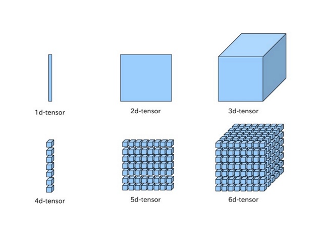
Terminology

Before we begin, let’s review the fundamental elements in PyTorch:

• Scalar: Single numerical value
  • 1, 2, 3
• Vector: 1-dimensional tensor
  • [1, 2, 3]
• Matrix: 2-dimensional tensor
  • [[1, 2, 3], [4, 5, 6]]
• Tensor: Multidimensional array (3 or more dimensions)
  • [[[1, 2, 3], [4, 5, 6]], [[7, 8, 9], [10, 11, 12]]]

Easy

Addition of Scalar and Vector

1 + torch.tensor([1, 2, 3]) # (1, ) + (3, )

Solution

"""
torch.tensor([1, 1, 1]) + torch.tensor([1, 2, 3])
"""
torch.tensor([2, 3, 4])

Explanation

• The scalar 1 of shape (1,) is broadcast to match the shape of the vector [1, 2, 3] of shape (3,), resulting in element-wise addition.

Addition between Matrices with Different Dimensions

x = torch.tensor([[1, 2, 3]]) # (1, 3)
y = torch.tensor([[1], [2], [3]]) # (3, 1)
x + y # (1, 3) + (3, 1)

Solution

"""
1. torch.tensor([[1, 2, 3]]) + torch.tensor([[1, 1, 1], [2, 2, 2], [3, 3, 3]]) ; (1, 3) + (3, 3)
2. torch.tensor([[1, 2, 3], [1, 2, 3], [1, 2, 3]]) + torch.tensor([[1, 1, 1], [2, 2, 2], [3, 3, 3]]) ; (3, 3) + (3, 3)
"""
tensor([[2, 3, 4],
        [3, 4, 5],
        [4, 5, 6]])

Explanation

• Broadcast trailing dimension of y to (3, 3) to match the trailing dimension of x.
• Now that y is of shape (3, 3), broadcast x to (3, 3)

Multiplication of Vector and Matrix

x = torch.tensor([1, 2, 3]) # (3, )
y = torch.tensor([[1], [2], [3]]) # (3, 1)
x * y # (3, ) * (3, 1)

Solution

"""
1. torch.tensor([[1, 2, 3]]) * torch.tensor([[1], [2], [3]]) ; (1, 3) * (3, 1)
2. torch.tensor([[1, 2, 3]]) * torch.tensor([[1, 1, 1], [2, 2, 2], [3, 3, 3]]) ; (1, 3) * (3, 3)
3. torch.tensor([[1, 2, 3], [1, 2, 3], [1, 2, 3]]) * torch.tensor([[1, 1, 1], [2, 2, 2], [3, 3, 3]]) ; (3, 3) * (3, 3)
"""
tensor([[1, 2, 3],
        [2, 4, 6],
        [3, 6, 9]])

Explanation

• Broadcasting logic is same as addition except for multiplying the elements.

Subtraction of Vector and Matrix

x = torch.tensor([1, 2, 3]) # (3, )
y = torch.tensor([[1, 1, 1], [2, 2, 2]]) # (2, 3)
x - y # (3, ) - (2, 3)

Solution

"""
1. torch.tensor([[1, 2, 3]]) - torch.tensor([[1, 1, 1], [2, 2, 2]]) ; (1, 3) - (2, 3)
2. torch.tensor([[1, 2, 3], [1, 2, 3]]) - torch.tensor([[1, 1, 1], [2, 2, 2]]) ; (2, 3) - (2, 3)
"""
tensor([[ 0,  1,  2],
        [-1,  0,  1]])

Explanation

• Prepend 1 to x to make shape of (1, 3).
• x and y’s trailing dimensions (3) both match.
• Broadcast x to match the shape of (2, 3).

Multiplication of Scalar and Matrix

x = torch.tensor(3) # Scalar has no shape, thus ([])
y = torch.tensor([[1, 2], [3, 4]]) # (2, 2)
x * y # ([]) - (2, 2)

Solution

"""
1. torch.tensor([3]) * torch.tensor([[1, 2], [3, 4]]) ; (1, ) * (2, 2)
2. torch.tensor([[3]]) * torch.tensor([[1, 2], [3, 4]]) ; (1, 1) * (2, 2)
3. torch.tensor([[3, 3]]) * torch.tensor([[1, 2], [3, 4]]) ; (1, 2) * (2, 2)
4. torch.tensor([[3, 3], [3, 3]]) * torch.tensor([[1, 2], [3, 4]]) ; (2, 2) * (2, 2)
"""
tensor([[ 3,  6],
        [ 9, 12]])

Explanation

• Scalar x has no dimension therefore broadcast it to (1, ).
• Prepend 1 to x to match the shape of the matrix.
• x of shape (1, 1) is then broadcasted to (1, 2) to match the trailing dimension of y.
• Remaining dimension of x is broadcasted to 2 to match the dimesion of y and becomes a shape of (2, 2).

Medium

Addition of Vector and Matrix

x = torch.tensor([1, 2, 3]) # (3, )
y = torch.tensor([[1], [2], [3]]) # (3, 1)
x + y # (3, ) + (3, 1)

Solution

"""
1. torch.tensor([[1, 2, 3]]) + torch.tensor([[1], [2], [3]]) ; (1, 3) + (3, 1)
2. torch.tensor([[1, 2, 3]]) + torch.tensor([[1, 1, 1], [2, 2, 2], [3, 3, 3]]) ; (1, 3) + (3, 3)
3. torch.tensor([[1, 2, 3], [1, 2, 3], [1, 2, 3]]) + torch.tensor([[1, 1, 1], [2, 2, 2], [3, 3, 3]]) ; (3, 3) + (3, 3)
"""
tensor([[2, 3, 4],
        [3, 4, 5],
        [4, 5, 6]])

Explanation

• Prepend 1 to x (dimension of tensor with fewer dimensions) to make x and y equal length.
• Start at the trailing dimension, y of shape (3, 1) is broadcasted to match the shape of x and becomes (3, 3).
• Matrix x of shape (1, 3) is broadcasted to match the shape of y and becomes (3, 3).

Addition of Vector and 3D Matrix

x = torch.tensor([1, 2, 3]) # (3, )
y = torch.ones(2, 3, 3) # (2, 3, 3)
x + y # (3, ) + (2, 3, 3)

Solution

"""
1. torch.tensor([[[1, 2, 3]]]) + torch.tensor([[[1, 1, 1], [1, 1, 1], [1, 1, 1]], [[1, 1, 1], [1, 1, 1], [1, 1, 1]]]) ; (1, 1, 3) + (2, 3, 3)
2. torch.tensor([[[1, 2, 3], [1, 2, 3], [1, 2, 3]]]) + torch.tensor([[[1, 1, 1], [1, 1, 1], [1, 1, 1]], [[1, 1, 1], [1, 1, 1], [1, 1, 1]]]) ; (1, 3, 3) + (2, 3, 3)
3. torch.tensor([[[1, 2, 3], [1, 2, 3], [1, 2, 3]], [[1, 2, 3], [1, 2, 3], [1, 2, 3]]]) + torch.tensor([[[1, 1, 1], [1, 1, 1], [1, 1, 1]], [[1, 1, 1], [1, 1, 1], [1, 1, 1]]]) ; (2, 3, 3) + (2, 3, 3)
"""
tensor([[[2, 3, 4],
         [2, 3, 4],
         [2, 3, 4]],

        [[2, 3, 4],
         [2, 3, 4],
         [2, 3, 4]]])

Explanation

• Prepend 1 twoce to x (dimension of tensor with fewer dimensions) to make x and y equal length (x now becomes (1, 1, 3)).
• First trailing dimensions of x and y match.
• x of shape (1, 1, 3) is broadcasted to (1, 2, 3) match the second trailing dimension of y.
• x is finally broadcasted to (2, 2, 3) and matches y’s dimension.

Addition of Two Matrices

x = torch.tensor([[1, 2, 3], [4, 5, 6]]) # (2, 3)
y = torch.tensor([[1, 2, 3, 4], [5, 6, 7, 8], [9, 10, 11, 12]]) # (3, 4)
x + y # (2, 3) + (3, 4)

Solution

---------------------------------------------------------------------------
RuntimeError                              Traceback (most recent call last)
<ipython-input-8-cd60f97aa77f> in <cell line: 1>()
----> 1 x + y

RuntimeError: The size of tensor a (3) must match the size of tensor b (4) at non-singleton dimension 1

Explanation

• Addition of x & y should fail as it violates the broadcasting semantics.
• One of following should hold according to the broadcasting semantics, starting at the trailing dimensions (i.e., x: 3 and y: 4):
  • Dimension sizes must equal
  • One of them is 1
  • One of them does not exist

Custom Dimension Manipulation

# Try to manipulate the dimension of `x` to make both compatible for addition
# HINT: `torch.Tensor.view`
x = torch.tensor([[1, 2, 3], [4, 5, 6]]) # (2, 3)
y = torch.tensor([[1, 2, 3, 4, 5, 6], [7, 8, 9, 10, 11, 12], [13, 14, 15, 16, 17, 18]]) # (3, 6)
x + y # (2, 3) + (3, 6)

Solution

"""
1. x.view(-1): torch.tensor([1, 2, 3, 4, 5, 6])
2. torch.tensor([1, 2, 3, 4, 5, 6]) + torch.tensor([[1, 2, 3, 4, 5, 6], [7, 8, 9, 10, 11, 12], [13, 14, 15, 16, 17, 18]]) ; (6, ) + (3, 6)
3. 2. torch.tensor([[1, 2, 3, 4, 5, 6]]) + torch.tensor([[1, 2, 3, 4, 5, 6], [7, 8, 9, 10, 11, 12], [13, 14, 15, 16, 17, 18]]) ; (1, 6) + (3, 6)
4. torch.tensor([[1, 2, 3, 4, 5, 6], [1, 2, 3, 4, 5, 6], [1, 2, 3, 4, 5, 6]]) + torch.tensor([[1, 2, 3, 4, 5, 6], [7, 8, 9, 10, 11, 12], [13, 14, 15, 16, 17, 18]]) ; (3, 6) + (3, 6)
"""
x = x.view(-1) # (6, )
x + y # (6, ) + (3, 6)

tensor([[ 2,  4,  6,  8, 10, 12],
        [ 8, 10, 12, 14, 16, 18],
        [14, 16, 18, 20, 22, 24]])

Explanation

• x.view(-1) transforms the dimension to (6, ).
• Prepends 1 to x and makes the dimension to (1, 6).
• Trailing dimension of both x and y (i.e, 6) matches.
• x’s 1 matches y’s dimension 3.

Multiplication of Complex Broadcasting

# Since it is a multiplication of `1`, try to answer the shape of this operation.
x = torch.ones(2, 1, 3) # (2, 1, 3)
y = torch.ones(1, 3, 1) # (1, 3, 1)
x * y # (2, 1, 3) * (1, 3, 1)

Solution

# Shape: (2, 3, 3)
tensor([[[1., 1., 1.],
         [1., 1., 1.],
         [1., 1., 1.]],

        [[1., 1., 1.],
         [1., 1., 1.],
         [1., 1., 1.]]])

Explanation

• Starting with shapes (2, 1, 3) and (1, 3, 1), let’s analyze dimension by dimension:
  1. First dimension: 2 vs 1 → y is broadcast from 1 to 2
  2. Middle dimension: 1 vs 3 → x is broadcast from 1 to 3
  3. Last dimension: 3 vs 1 → y is broadcast from 1 to 3
• Final shapes before multiplication:
  • x: (2, 3, 3) (original 1 expanded to 3 in middle)
  • y: (2, 3, 3) (expanded from 1 to 2 in first, and 1 to 3 in last)
• Since all elements are 1, the multiplication results in a (2, 3, 3) tensor of ones

Hard

Mean Across Specific Axes

# Compute the mean of the x across the last axis, and add it back to the original tensor
g = torch.Generator().manual_seed(617) # guarantees consistent random generation
x = torch.rand(3, 4, 5, generator=g)

Solution

x + x.mean(dim=2, keepdims=True)

# <--- OUTPUT --->
tensor([[[0.5952, 0.6486, 1.1932, 0.4631, 1.1062],
         [0.7727, 0.9813, 0.4742, 0.6173, 1.0093],
         [0.5897, 0.6357, 0.8125, 0.8716, 0.4222],
         [1.1211, 0.4338, 0.6372, 0.4942, 0.7857]],

        [[0.6572, 1.3236, 1.3613, 0.4812, 0.5334],
         [1.5122, 1.1478, 1.1528, 1.4942, 0.7012],
         [1.1803, 1.4021, 1.4673, 1.1307, 0.9080],
         [1.6144, 0.6951, 1.1600, 1.2778, 1.5087]],

        [[1.3744, 0.9883, 0.6701, 1.1222, 1.1225],
         [0.9468, 0.8783, 0.4040, 0.6899, 1.0623],
         [1.2763, 1.0732, 0.7736, 1.5029, 0.5423],
         [1.0240, 1.2803, 1.1804, 1.5658, 0.9504]]])

# Verify
first_row = x[0][0] # torch.tensor([0.1946, 0.2479, 0.7926, 0.0624, 0.7056]) ; (5, )
first_row_mean = x[0][0].mean() # torch.tensor(0.4006) ; ([])
result = first_row + first_row_mean
matches = result == (x + x.mean(dim=2, keepdims=True))[0][0]

print(result)
print(matches)

# <--- OUTPUT --->
tensor([0.5952, 0.6486, 1.1932, 0.4631, 1.1062])
tensor([True, True, True, True, True])

Explanation

• The original tensor x has shape (3, 4, 5)
• x.mean(dim=2, keepdims=True) does the following:
  1. Computes the mean along dimension 2 (the last axis)
  2. keepdims=True preserves the dimension, resulting in shape (3, 4, 1)
  3. When adding this back to x, broadcasting expands the mean from (3, 4, 1) to (3, 4, 5)
• Each element in the result is the sum of:
  1. The original value from x
  2. The mean of its corresponding row (broadcast across the last dimension)
• The verification code confirms this by:
  1. Taking the first row x[0][0] (shape (5,))
  2. Adding its mean (a scalar) to each element
  3. Comparing with the corresponding row in the full calculation

Broadcasting with Max Reduction

# Find the maximum value of each row and subtract this value from the original tensor.
g = torch.Generator().manual_seed(617)
x = torch.rand(4, 3, 2, generator=g)

Solution

max_rows = x.max(dim=2, keepdims=True).values # (4, 3, 1)
x - max_rows # (4, 3, 2) - (4, 3, 1)

# <--- OUTPUT --->
tensor([[[-0.0533,  0.0000],
         [ 0.0000, -0.7302],
         [ 0.0000, -0.3184]],

        [[ 0.0000, -0.5071],
         [-0.3920,  0.0000],
         [-0.0460,  0.0000]],

        [[-0.0591,  0.0000],
         [-0.6848,  0.0000],
         [-0.2034,  0.0000]],

        [[-0.2914,  0.0000],
         [-0.6664,  0.0000],
         [ 0.0000, -0.8801]]])

Explanation

• The original tensor x has shape (4, 3, 2)
• x.max(dim=2, keepdims=True)[0] does the following:
  1. Takes the maximum value along dimension 2 (last axis) for each row
  2. keepdims=True maintains the dimension, resulting in shape (4, 3, 1)
  3. [0] is used because max() returns both values and indices; we only want values
• When subtracting maxOfRows from x, broadcasting expands (4, 3, 1) to (4, 3, 2)
• The result shows each value’s difference from its row’s maximum:
  • Values equal to their row’s maximum become 0
  • All other values are negative (being less than their row’s maximum)

Combining Argmax with Tensor Indexing

"""
Compute argmax of `x` along dim=2, then replace the maximum values along that dimension with their square while keeping other values unchanged.
"""
g = torch.Generator().manual_seed(617)
x = torch.rand(5, 4, 6, generator=g)

Solution

indices = x.argmax(dim=2) # (5, 4)

mask = torch.zeros_like(x, dtype=torch.bool)
batch_indices = torch.arange(x.size(0)).unsqueeze(1)  # (5, 1)
row_indices = torch.arange(x.size(1)).unsqueeze(0)    # (1, 4)
mask[batch_indices, row_indices, indices] = True

x = torch.where(mask, x ** 2, x)

# <--- OUTPUT --->
tensor([[[1.9459e-01, 2.4792e-01, 6.2822e-01, 6.2441e-02, 7.0561e-01,
          3.8723e-01],
         [5.9580e-01, 8.8707e-02, 2.3185e-01, 3.8913e-01, 2.5649e-01,
          3.0251e-01],
         [4.7937e-01, 5.3843e-01, 8.9037e-02, 5.9889e-01, 8.6632e-02,
          2.9001e-01],
         [1.4702e-01, 4.3846e-01, 2.2150e-01, 8.8794e-01, 8.5682e-01,
          4.5569e-02]],

        [[9.7745e-02, 8.3054e-01, 5.4700e-01, 5.5202e-01, 8.9336e-01,
          1.0040e-01],
         [5.7145e-01, 7.9327e-01, 8.5845e-01, 5.2186e-01, 2.9914e-01,
          9.7775e-01],
         [6.9493e-02, 5.3443e-01, 6.5223e-01, 7.7981e-01, 8.4665e-01,
          4.6055e-01],
         [1.4233e-01, 5.9448e-01, 3.5373e-01, 5.4865e-01, 4.8015e-01,
          5.8755e-03]],

        [[2.9175e-01, 6.6421e-01, 7.5952e-01, 5.5636e-01, 2.5674e-01,
          9.7236e-01],
         [2.5453e-02, 4.2386e-01, 6.8020e-01, 5.8032e-01, 9.3263e-01,
          3.5035e-01],
         [1.4200e-01, 1.2870e-01, 3.0852e-01, 1.0691e-01, 2.1062e-01,
          1.7581e-02],
         [5.7376e-01, 1.3413e-01, 5.2298e-01, 9.0579e-02, 6.6662e-01,
          9.5560e-01]],

        [[3.7499e-01, 7.5693e-01, 7.9677e-01, 5.3703e-01, 6.5874e-01,
          6.6973e-01],
         [5.4903e-01, 7.6660e-01, 2.5739e-01, 6.2306e-01, 3.9811e-01,
          3.2552e-01],
         [9.6114e-02, 6.8212e-01, 9.9059e-01, 8.4072e-01, 5.6158e-01,
          4.1336e-01],
         [2.9504e-01, 1.7929e-01, 3.7160e-01, 1.4645e-01, 1.4089e-01,
          3.6650e-01]],

        [[7.9860e-01, 1.6316e-01, 7.0585e-01, 7.4827e-01, 7.2970e-01,
          3.8324e-01],
         [3.9089e-01, 5.9064e-01, 8.0657e-01, 1.7587e-01, 3.3804e-01,
          1.9550e-01],
         [7.8799e-01, 3.3231e-01, 7.0377e-02, 8.0018e-01, 5.0456e-01,
          9.6001e-01],
         [5.4405e-01, 8.8870e-01, 3.7259e-04, 8.8793e-01, 6.1661e-01,
          8.4178e-01]]])

Explanation

1. First, find the indices of maximum values along dimension 2:
   • x.argmax(dim=2) returns a tensor of shape (5, 4) containing the positions of max values
2. Create a boolean mask of the same shape as x (5, 4, 6):
   • torch.zeros_like(x, dtype=torch.bool) initializes all values to False
3. Create broadcasting-compatible indices to properly index the 3D tensor:
   • batch_indices = torch.arange(5).unsqueeze(1) creates [[0], [1], [2], [3], [4]]
   • row_indices = torch.arange(4).unsqueeze(0) creates [[0, 1, 2, 3]]
   • When used together, these broadcast to cover all positions where max values occur
4. Set True in the mask at positions of maximum values:
   • mask[batch_indices, row_indices, indices] = True
   • The indexing operation mask[batch_indices, row_indices, indices] works through broadcasting:

     batch_indices: [[0],    # Shape: (5, 1)
                    [1],
                    [2],
                    [3],
                    [4]]
     
     row_indices:   [[0, 1, 2, 3]]    # Shape: (1, 4)
     
     indices:       [[2, 3, 3, 4],     # Shape: (5, 4)
                    [1, 5, 3, 2],
                    [5, 4, 0, 5],
                    [4, 3, 2, 4],
                    [3, 2, 5, 1]]
     

   • When combined, these create index tuples for each maximum value:
     • First row: (0,0,2), (0,1,3), (0,2,3), (0,3,4)
     • Second row: (1,0,1), (1,1,5), (1,2,3), (1,3,2)
     • And so on.
   • Each tuple represents (batch_idx, row_idx, max_value_position)
5. Finally, torch.where() selectively applies the squaring:
   • Where mask is True: square the values (x ** 2)
   • Where mask is False: keep original values (x)

Comparing Reduction Results Across Axes

# Compute max along dim=2 and mean along dim=1 and add those results back to the original tensor
g = torch.Generator().manual_seed(617)
x = torch.rand(3, 4, 5, generator=g)

Solution

max_dim2 = x.max(dim=2, keepdim=True).values # (3, 4, 1)
mean_dim1 = x.mean(dim=1, keepdim=True) # (3, 1, 5)

result = x + max_dim2 + mean_dim1 # (3, 4, 5) + (3, 4, 1) + (3, 1, 5)

# <--- OUTPUT --->
tensor([[[1.3902, 1.3487, 1.9979, 1.1000, 1.9624],
         [1.4141, 1.5278, 1.1252, 1.1006, 1.7118],
         [1.1980, 1.1492, 1.4305, 1.3218, 1.0917],
         [1.9508, 1.1687, 1.4766, 1.1658, 1.6766]],

        [[1.8204, 2.3880, 2.5689, 1.4995, 1.3685],
         [2.4959, 2.0328, 2.1810, 2.3330, 1.3568],
         [2.1032, 2.2261, 2.4345, 1.9086, 1.5027],
         [2.6509, 1.6327, 2.2409, 2.1693, 2.2170]],

        [[2.3380, 1.8515, 1.2353, 2.1506, 1.8501],
         [1.8575, 1.6887, 0.9164, 1.6655, 1.7371],
         [2.3903, 2.0868, 1.4891, 2.6817, 1.4202],
         [2.0343, 2.1902, 1.7924, 2.6410, 1.7248]]])

Explanation

• The original tensor x has shape (3, 4, 5)
• Two reduction operations are performed:
  1. max_dim2: Maximum along dimension 2 (last axis)
     • Shape goes from (3, 4, 5) → (3, 4, 1) with keepdim=True
     • Each value represents the maximum of its corresponding row
  2. mean_dim1: Mean along dimension 1 (middle axis)
     • Shape goes from (3, 4, 5) → (3, 1, 5) with keepdim=True
     • Each value represents the mean across all rows for that position
• The final addition x + max_dim2 + mean_dim1 involves two broadcasting operations:
  • max_dim2 (3, 4, 1) is broadcast to (3, 4, 5)
  • mean_dim1 (3, 1, 5) is broadcast to (3, 4, 5)

Standardizing Tensor with Reduction

# Standardize x along the last axis (dim=2) by subtracting the mean and dividing by the standard deviation.
g = torch.Generator().manual_seed(617)
x = torch.rand(3, 5, 4, generator=g)

Solution

mean = x.mean(dim=2, keepdims=True) # (3, 5, 1)
std = x.std(dim=2, keepdims=True) # (3, 5, 1)

result = (x - mean) / std # (3, 5, 4) - (3, 5, 1) / (3, 5, 1)

# <--- OUTPUT --->
tensor([[[-4.0344e-01, -2.3768e-01,  1.4553e+00, -8.1418e-01],
         [ 9.6276e-01, -2.1043e-01,  5.5813e-01, -1.3105e+00],
         [-6.6763e-01,  1.4806e+00, -5.3258e-01, -2.8035e-01],
         [ 3.2340e-02,  2.4018e-01, -1.3413e+00,  1.0688e+00],
         [-9.7956e-01,  3.1494e-01, -5.9517e-01,  1.2598e+00]],

        [[-6.6012e-01,  8.1287e-01,  8.9620e-01, -1.0490e+00],
         [-1.2885e+00,  1.1535e+00,  5.9946e-02,  7.5018e-02],
         [ 8.6095e-01, -1.3867e+00, -5.1503e-02,  5.7724e-01],
         [ 6.0867e-01, -4.6181e-01, -1.1701e+00,  1.0233e+00],
         [-1.3592e+00, -1.0854e-03,  3.4300e-01,  1.0173e+00]],

        [[ 1.1443e+00, -1.7200e-01, -1.2569e+00,  2.8459e-01],
         [ 6.8955e-01,  5.1992e-01,  2.6785e-01, -1.4773e+00],
         [-1.3675e+00,  4.7652e-01,  9.4842e-01, -5.7411e-02],
         [-4.0622e-01,  1.3754e+00, -9.7121e-01,  2.0231e-03],
         [ 1.4138e-01, -2.5028e-01,  1.2610e+00, -1.1521e+00]]])

Conclusion

We have learned about broadcasting semantics and how to use them to perform various operations on tensors.

Remeber the basic rules of broadcasting:

• Each tensor has at least one dimension.
• When iterating over the dimension sizes, starting at the trailing dimension, the dimension sizes must either be equal, one of them is 1, or one of them does not exist.

Broadcasting is a powerful feature that allows us to perform operations on tensors of different shapes without explicitly reshaping them. It is a key concept in PyTorch and is used extensively in many operations. And this will help us in the next post to build character-level bigram models.