Bengio: A Neural Probabilistic Language Model

Introduction

This time, we will skim through Yoshua Bengio’s seminal paper A Neural Probabilistic Language Model (2003) which laid the foundation of:

• Statistical language modeling that addressed the curse of dimensionality.
• Word Embedding representations allowing to capture the semantic and syntatic similarities between words.
• Neural network based language models that paved the way for modern transformer models.

We will expand our previous character-level language model to a trigram model by adopting the model architecture proposed in the paper.

Paper Overview

Let’s briefly go over the points made by Bengio in the paper.

Curse of Dimensionality

In machine learning, curse of dimensionality refers to a phenomenon where the number of features or dimensions in the dataset grows exponentially as the number of samples grows linearly. As dimensionality increases, data becomes sparse and the amount of data required to generalize accurately increases exponentially.

Think of a case if one wants to model the joint probability of 10 consecutive words in English with a vocabulary V of size 100,000. The number of possible combinations is $100,000^{10} = 10^{50}$ with potential free parameters of ${100,000}^{10} - 1 = 10^{50} - 1$ (Remember the normalization constraint that probabilities must sum to 1). This is an astronomically large number, far beyond the reach of any computer.

Discrete vs. Continuous Representations

N-gram models use discrete representation for words, which harms the generalization of the model. Any change in the variable may lead to a drastic change in the probability distribution (e.g., dog & dogs might be assigned drastically different probabilities). Meanwhile, it is easier to obtain generalization using continuous representations. Smooth classes of functions, such as those used in neural network-based language models (e.g., word embeddings in vector spaces), allow for small changes in input to result in small changes in output, leading to better generalization and robustness to variations in language.

Problems Raised by the Bengio

1. Short Context Window

   N-gram models, which are typically trigram models (n=3), have limiting context window which ignores the long-range dependencies in the language. A sentence “She saw a bank robbery.”, might be problematic for a trigram model since:

   • Ambiguity in “bank”: “bank” could be a financial institution or a body of water.
   • Limited Context Window: The model might assign a place (e.g., river) next to the three-word sequence “She saw a bank” which is more likely than a word “robbery”.

2. Data Sparsity

   Although there are alternative model smoothing approaches such as Katz Backoff or Interpolation to obtain the sequence probabilities using smaller context windows, the model is still limited by the size of the context window. Therefore, even with these smoothing techniques, the model is still the victim of curse of dimensionality.

3. Lack of Syntactic and Semantic Similarities

   

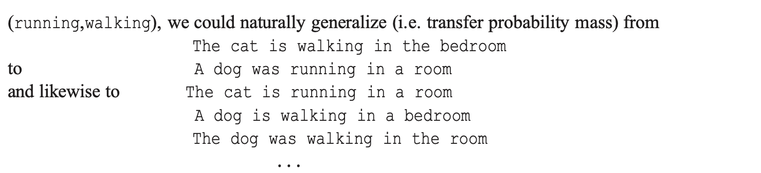
   N-gram model fail to take similarities between words into account. For example, "The cat is walking in the bedroom in the training corpus should be able to generate sentence like "The dog is running in the kitchen" since there are semantic similarities between cat and dog and bedroom and kitchen. However, N-gram model will assign low probabilities to these sentences since the context window is too small to capture these relationships.

Embedding to Capture Syntactic and Semantic Similarities

In order to tackle the above problems (especially the third one), Bengio proposed a neural network based language model that uses embedding to capture the syntactic and semantic similarities between words.

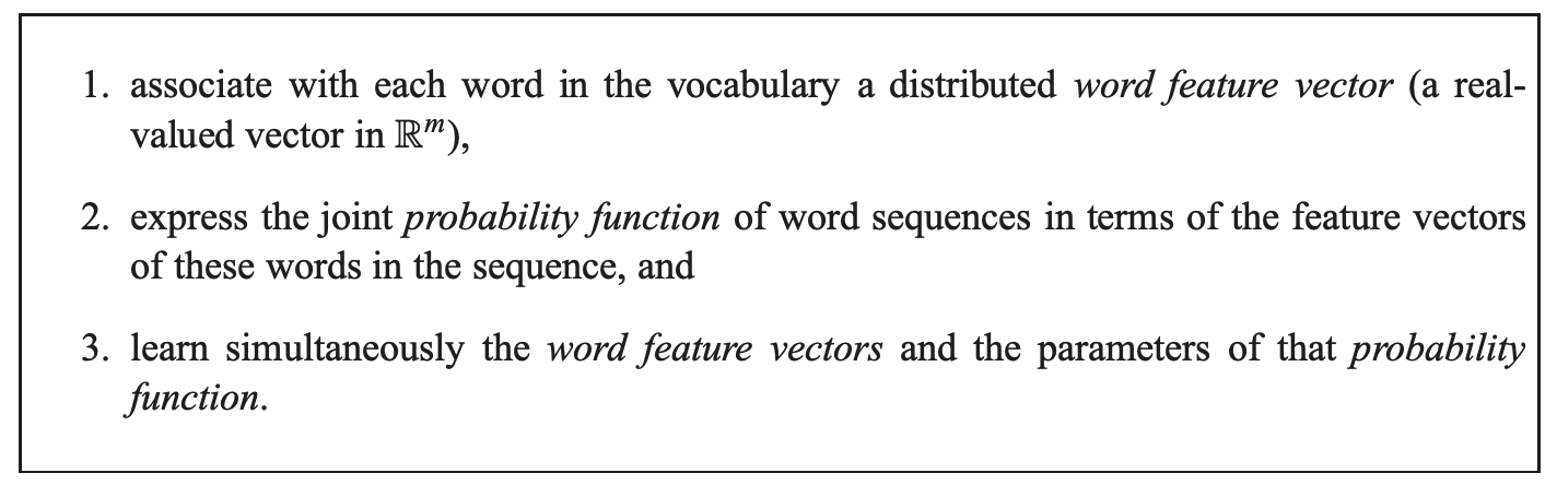
Steps above explained in more modern-day lingo:

1. Create a lookup table to map each word to a unique integer index.
   • Each word in the vocabulary is mapped to a real-valued vector $w_i \in \mathbb{R}^m$, where $m$ is the embedding dimension (e.g., $m = 30, 60$).
   • Words are now expressed as dense vectors in a continuous vector space.
   • Words with similar meanings will have similar vectors.
2. Learn the Joint Probability Function Using the Word Embedding
   • The model expresses the joint probability of a sequence of words in terms of embeddings of the words.
   • The neural network takes as input the current and previous words in the sentence and outputs the probability of the next word.
3. Train the model and embedding via backpropagation
   • The model and embedding are trained via backpropagation.
   • The model is trained to maximize the likelihood (or minimize the negative likelihood) of the training data.
   • The embedding is trained to capture the syntactic and semantic similarities between words.

Model Architecture

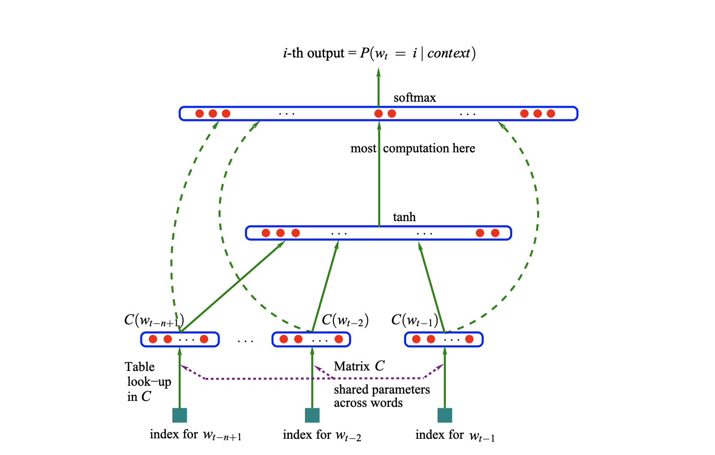
For our implementation, we will use the following notations:

• $w_{1:t} \in V$: Training sequence of words that are in finite vocabulary set $V$.
• $f(w_t, w_{t-1}, \ldots, w_{t-n+1}) = \hat{P}(w_t \mid w_{t-1}, \ldots, w_{t-n+1})$: Objective function to learn the joint probability of the training sequence.
• $C(i) \in \mathbb{R}^{m}$: Look-up table for character: (27, 10)
• $W_1 \in \mathbb{R}^{m \times h}$: Weight matrix for the hidden layer (accounting for the concatenated embedding): (30, 200)
• $b_1 \in \mathbb{R}^{h}$: Bias vector for the hidden layer: (200,)
• $W_2 \in \mathbb{R}^{h \times V}$: Weight matrix for the output layer: (200, 27)

• $b_2 \in \mathbb{R}^{V}$: Bias vector for the output layer: (27,)

• We are using block_size = 3 for the trigram model, and when linearly transforming the embedding, we will be concatenating the the input vectors into a single vector of size m * block_size.
• Therefore, the size of the weight matrix for the hidden layer will be (m * block_size, h).
• The output matrix will be size of the finite character set, 27.
• Keep in mind that the actual implementation uses mini-batch training therefore the size of the output matrix will be (batch_size, 27).

Implementation

Build itos & stoi table

Same as the previous post, we build the itos & stoi tables to map each character to a unique integer index and vice versa.

# Build itos & stoi table
chars = sorted(list(set(''.join(w for w in words))))
stoi = {c : (idx + 1) for idx, c in enumerate(chars)}
stoi['.'] = 0

itos = {v : k for k, v in stoi.items()}
vocab_size = len(itos)

Build train, validation, and test dataset

In machine learning, we often split the dataset into train, validation, and test sets. Each set is used for different purposes:

• Train Set: Used to train the model. The dataset is used to adjust weights and biases of the model.
• Validation Set: Validation set is still involved in the training process. It is used to tune the hyperparameters and to select the best model.
• Test Set: Used to evaluate the performance of the model. It is not used to adjust the weights and biases of the model, or to tune the hyperparameters. It is soely used to evaluate the performance of the model.

block_size = 3

# Create Dataset
def build_dataset(words):
    X, Y = [], []

    for word in words:
        context = [0] * block_size

        for char in word + '.':
            ix = stoi[char]

            X.append(context)
            Y.append(ix)

            context = context[1:] + [ix]

    X = torch.tensor(X)
    Y = torch.tensor(Y)

    print(X.shape, Y.shape)

    return X, Y

import random
random.seed(42)
random.shuffle(words)

n1 = int(0.8 * len(words))
n2 = int(0.9 * len(words))

Xtr, Ytr = build_dataset(words[:n1]) # Train: 80%
Xval, Yval = build_dataset(words[n1:n2]) # Validation: 10%
Xtest, Ytest = build_dataset(words[n2:]) # Test: 10%

torch.Size([182771, 3]) torch.Size([182771])
torch.Size([22711, 3]) torch.Size([22711])
torch.Size([22664, 3]) torch.Size([22664])

Initialize the Parameters

Refer to the model architecture section for the size of the parameters. Parameters such as n_embd and n_hidden are hyper-parameters that can be tuned during the training process.

n_embd = 10 # the dimensionality of the character embedding vectors
n_hidden = 200 # the number of neurons in the hidden layer of the MLP

g = torch.Generator().manual_seed(2147483647)

C = torch.randn((vocab_size, n_embd), generator=g) # look-up table for character: (27, 10)
W1 = torch.randn((n_embd * block_size, n_hidden), generator=g) # hidden layer for the concatenated trigram: (30, 200)
b1 = torch.randn(n_hidden, generator=g) # (200, )
W2 = torch.randn((n_hidden, vocab_size), generator=g) # (200, 27)
b2 = torch.randn(vocab_size, generator=g)

parameters = [C, W1, W2, b1, b2]
for p in parameters:
    p.requires_grad = True

# arrays to plot the loss per learning rate
lre = torch.linspace(-3, 0, 1000) # Generates 1000 evenly spaced numbers between -3 and 0
lrs = 10**lre # learning rates raised 10 to the power of lre

lri = []
lossi = []
stepi = []

Training Loop

The training loop is the core of the model. It is where the model learns the patterns in the data.

Lines to note:

• ix = torch.randint(0, Xtr.shape[0], (batch_size, ), generator=g): Randomly select a batch of data.
• Xb, Yb = Xtr[ix], Ytr[ix]: Gets the batch of data.
• emb = C[Xb]: Gets the embedding of the batch of data using fancy indexing.
• h = torch.tanh(emb.view(-1, 30) @ W1 + b1): Concatenates the input data into a single matrix and applies the linear transformation.
• logits = h @ W2 + b2: Applies the linear transformation to the hidden layer and adds the bias.
• loss = F.cross_entropy(logits, Yb): Get the loss of the batch of data.

# Training Loop
epochs = 200000
batch_size = 32

# Mini-Batch Training
for epoch in range(epochs):
    ix = torch.randint(0, Xtr.shape[0], (batch_size, ), generator=g) # Randomly select a batch of data
    Xb, Yb = Xtr[ix], Ytr[ix]

    emb = C[Xb]
    h = torch.tanh(emb.view(-1, 30) @ W1 + b1)
    logits = h @ W2 + b2
    loss = F.cross_entropy(logits, Yb)

    for p in parameters:
        p.grad = None
    loss.backward()

    lr = 0.1 if epoch < 10000 else 0.01
    for p in parameters:
        p.data += -lr * p.grad
    
    if epoch % 10000 == 0:
        print(f'{epoch}: {loss.item():.4f}')
    
    lossi.append(loss.log10().item())
    stepi.append(epoch)

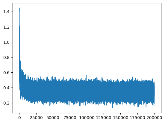
The loss of the training set quickly decreases from the 0-th epoch to the 10000-th epoch and starts converging. You can check that the loss graph below looks like a hockey stick. We will be covering a technique to normalize the loss in the later post (Weight Initialization & Batch Normalization).

0: 25.3725
10000: 2.5161
20000: 2.3014
30000: 2.3739
40000: 2.7937
50000: 2.3582
60000: 2.5736
70000: 2.7811
80000: 2.0506
90000: 2.3116
100000: 2.4187
110000: 2.2202
120000: 1.6289
130000: 2.3359
140000: 2.4920
150000: 2.4063
160000: 2.1622
170000: 2.0637
180000: 2.0356
190000: 1.9934

plt.plot(stepi, lossi)

Compute the Loss

You can see that the computed loss of training, validation and test are all close to each other. This is a good sign that the model is generalizing well.

# Train Loss
emb = C[Xtr]
h = torch.tanh(emb.view(-1, 30) @ W1 + b1)
logits = h @ W2 + b2
loss = F.cross_entropy(logits, Ytr)
print(loss)

# Valid Loss
emb = C[Xval]
h = torch.tanh(emb.view(-1, 30) @ W1 + b1)
logits = h @ W2 + b2
loss = F.cross_entropy(logits, Yval)
print(loss)

# Test Loss
emb = C[Xtest]
h = torch.tanh(emb.view(-1, 30) @ W1 + b1)
logits = h @ W2 + b2
loss = F.cross_entropy(logits, Ytest)
print(loss)

tensor(2.2249, grad_fn=<NllLossBackward0>)
tensor(2.2488, grad_fn=<NllLossBackward0>)
tensor(2.2542, grad_fn=<NllLossBackward0>)

Conclusion

That’s it for this post! We have adopted Bengio’s Neural Probabilistic Language Model to build a character-level trigram model. We have also covered the following:

• Weakness of N-gram models:
  • Long term dependencies are not captured.
  • Data sparsity.
  • Lack of syntactic and semantic similarities.
• Neural Network based language models:
  • Embedding to capture syntactic and semantic similarities.
  • Model that generalizes well to unseen data.
• Train, Validation, and Test Sets
• Mini-Batch Training
• Cross-Entropy Loss
• Potential Improvements to prevent drastic loss changes:
  • Weight Initialization
  • Batch Normalization