Weight Initialization of Neural Networks

Introduction

Weights and biases one of the most important factors of neural networks. Think about all the topics (e.g., backpropagation, activation functions, loss functions, optimization, regularization, etc.) we have covered so far. Each and every one of them was in pursuit of finding the best weights and biases that best fit the data.

So far, we have assumed that the weights and biases are initialized randomly. Pretty much the entire weight and bias initialization code looked like this:

W = np.random.randn((input_dim, output_dim)).float()
b = np.random.randn((output_dim,)).float()

And this wasn’t necessarily wrong. How else should the parameters be initialized in the first place? Well, there are actually a few ways to initialize the parameters (depending on the activation function of the hidden layer). In this post, we will cover two of the most popular initialization methods: Xavier Initialization and Kaiming He Initialization.

Problem with Random Initialization

Let’s first review the trigram model that we have implemented in the previous post. We performed a mini-batch training by:

• Pluck out 3 character embeddings from the look-up table and concatenate into a single vector (therefore making the embedding dimension from 10 to 30).
• Apply a non-linear activation function and calculate logits by multiplying the concatenated vector with the weight matrix and adding the bias.
• Compute the loss between the predicted and the actual character.
• Backpropagate the loss to update the weights and biases.

The paramters are initialized as follows:

n_embd = 10 # the dimensionality of the character embedding vectors
n_hidden = 200 # the number of neurons in the hidden layer of the MLP
vocab_size = 27 # the number of characters in the vocabulary
block_size = 3 # the number of characters in the input sequence

g = torch.Generator().manual_seed(2147483647) # for reproducibility
C  = torch.randn((vocab_size, n_embd),            generator=g)
W1 = torch.randn((n_embd * block_size, n_hidden), generator=g)
b1 = torch.randn(n_hidden,                        generator=g) 
W2 = torch.randn((n_hidden, vocab_size),          generator=g) 
b2 = torch.randn(vocab_size,                      generator=g)

The loss of the training loop is as follows:

for epoch in range(200000):
    # minibatch construct
    ix = torch.randint(0, Xtr.shape[0], (32,))
    Xb, Yb = Xtr[ix], Ytr[ix]

    # forward pass
    emb = C[Xb] # (32, 3, 2)
    embcat = emb.view(emb.shape[0], -1)
    hpreact = embcat @ W1 + b1
    h = torch.tanh(hpreact) # (32, 100)
    logits = h @ W2 + b2 # (32, 27)
    loss = F.cross_entropy(logits, Ytr[ix])

    # backward pass
    for p in parameters:
        p.grad = None
    loss.backward()

    # update
    #lr = lrs[i]
    lr = 0.1 if epoch < 100000 else 0.01
    for p in parameters:
        p.data += -lr * p.grad

    if epoch % 100000 == 0:
        print(f'{epoch}: {loss.item()}')

    # track stats
    #lri.append(lre[i])
    stepi.append(epoch)
    lossi.append(loss.log10().item())

0: 25.3725
10000: 2.5161
20000: 2.3014
30000: 2.3739
40000: 2.7937
50000: 2.3582
60000: 2.5736
70000: 2.7811
80000: 2.0506
90000: 2.3116
100000: 2.4187
110000: 2.2202
120000: 1.6289
130000: 2.3359
140000: 2.4920
150000: 2.4063
160000: 2.1622
170000: 2.0637
180000: 2.0356
190000: 1.9934

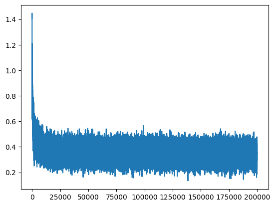
The loss of the training set quickly decreases from 25.3725 to 2.5161 at the 10000-th epoch and start converging. Hockey-stick look alike graph also indicates such a sharp decrease in the loss.

What loss should we be expecting from the model in the initialization step? Since the parameters are not trained yet, the model should assign equal probability (i.e., 1/27 or loss of -log(1/27) = 3.2958) to each character.

Therefore, the loss of 25.3725 indicates that the model is confidently assigning wrong probability distribution to the characters. And this is where the problem with random initialization comes from.

Example: Extreme Softmax Leads to Extreme Loss

We will go through a few examples to see how different logits result in different softmax probabilities and, consequently, different losses.

For those who are not familiar with softmax, softmax is a function that converts a vector of real numbers into a vector of probability distributions.

Given an input vector $z = [z_1, z_2, z_3, …, z_n]$, the mathematical formula is as follows:

\[\text{softmax}(z_i) = \frac{e^{z_i}}{\sum_{j=1}^{n} e^{z_j}}\]

Or, to prevent numerical overflow and underflow, the softmax function is often rewritten as below for numerical stability:

\[\text{softmax}(z_i) = \frac{e^{z_i - \max(z)}}{\sum_{j=1}^{n} e^{z_j - \max(z)}}\]

Here are some of important properties of softmax function:

• Normalizes the logits to a probability distribution.
• The value of each element of the output vector is in the range of [0, 1].
• The sum of the output vector is 1.

As mentioned from the Negative Log Likelihood Explained, we will be covering more about softmax and cross-entropy loss in the future.

Case 1: Equal Logits and Softmax Probabilities

logits = torch.tensor([0.25, 0.25, 0.25, 0.25])
probs = torch.softmax(logits, dim=0)

# Loss of the correct class
loss = -probs[2].log()
print("probs:", probs)
print("loss:", loss)

probs: tensor([0.2500, 0.2500, 0.2500, 0.2500])
loss: tensor(1.3863)

In this case, the model assigns equal probability to each character and thus has a NLL loss of 1.3863. And not surprisingly, the loss of 1.3863 is constant as long as the distribution of the logits is identical (e.g, logits = torch.tensor([5.0, 5.0, 5.0, 5.0])).

Case 2: Logits with One Extremely Large Value

logits = torch.tensor([0.01, 64.00, 0.01, 0.01])
probs = torch.softmax(logits, dim=0)

# Loss of the correct class
loss = -probs[2].log()
print("probs:", probs)
print("loss:", loss)

probs: tensor([1.6199e-28, 1.0000e+00, 1.6199e-28, 1.6199e-28])
loss: tensor(63.9900)

This is an interesting case. The model confidently assigns a high probability to the incorrect class (i.e., 64.00 to index 1) and thus has a NLL loss of 63.9900 (which is close to the raw value of the incorrect logit).

Since 64.00 is much larger than the other logits, the exponentiation of each value leads to:

• $e^{64.00}$: 6.2351491e+27 or 6.23 * 10^27
• $e^{0.01}$: 1.0001

This makes $e^{64.00}$ dominate the denominator of the softmax function and thus makes other logits close to 0.

\[p_1 = \frac{e^{64.00}}{e^{64.00} + e^{0.01} + e^{0.01} + e^{0.01}} \approx 1\] \[p_2 = \frac{e^{0.01}}{e^{64.00} + e^{0.01} + e^{0.01} + e^{0.01}} \approx e^{-64.00} \approx 1.6199 * 10^{-28}\] \[\text{Since } \log(e) = 1,\] \[-log(p_2) = -log(1.6199 * 10^{-28}) = -log(e^{-64.00}) = 64.00\]

Case 3: Logits with Random Values Distributed Around Zero

torch.manual_seed(1)

logits = torch.randn(4)
probs = torch.softmax(logits, dim=0)

# Loss of the correct class
loss = -probs[2].log()
print("logits:", logits)
print("probs:", probs)
print("loss:", loss)

logits: tensor([0.6614, 0.2669, 0.0617, 0.6213])
probs: tensor([0.6614, 0.2669, 0.0617, 0.6213])
loss: tensor(1.7578)

This case has rather a balanced distribution of logits around zero. And despite the randomly generated values, the loss 1.7578 is not too far from the loss 1.3863 in the first case.

Case 4: Logits with Random Values of High Magnitude

torch.manual_seed(1)

logits = torch.randn(4) * 30
probs = torch.softmax(logits, dim=0)

# Loss of the correct class
loss = -probs[2].log()
print("logits:", logits)
print("probs:", probs)
print("loss:", loss)

logits: tensor([19.8406,  8.0077,  1.8503, 18.6395])
probs: tensor([7.6871e-01, 5.5824e-06, 1.1822e-08, 2.3129e-01])
loss: tensor(18.2533)

Now suppose that we multiplied the logits by 30. The more the logits are extreme, the more softmax probabilities are assigned due to the nature of exponential function. And now we see the sharp increase in the loss from 1.7578 to 18.2533. And this is the most likely scenario happening in the our trigram model too. The model in the initial phase is assigning extreme probabilities to the incorrect classes and thus leading to the loss of 25.3725.

Reduce the Magnitude of Weights and Biases by a Small Number

Before we dive into the details of Xavier and Kaiming He Initialization, let’s take a naive apporoach to reduce the magnitude of the weights and biases by a small number.

Taking a look at the first logits vector in the training loop, we have:

print(f'{i}: {loss.item()}')
print(logits[0]) # Calculated by `logits = h @ W2 + b2`

0: 25.3725
tensor([ 18.8867,  -2.0754,  -4.1544,  17.9570, -12.9605, -17.7149, -19.5287,
          2.9100,  20.1812,  -6.0030,  -6.9961,   8.2149,   6.2865, -16.9456,
         -0.5052,   4.0713, -14.4158,  13.4091,  14.9163, -14.7873,  -4.1053,
         -1.1352,   4.1154,  -2.2791,  -9.8275,   0.8839,  -0.6039],
       grad_fn=<SelectBackward0>)

You can see that the loss is quite high as the logits are quite large. This resembles the case 4 where the logits are of high magnitude. In order to have a relatively small loss, we should reduce the magnitude of the logits (as we have seen in case 3).

As the logits vector is calculated by h @ W2 + b2, we can do the following:

Set b2 to 0

Bias shifts the activation function (more specifically, the product of input and weight) by a constant value. Neurons will receive different input and weights, thus eventually diverge even if the biases are set to zero.

b2 = torch.randn(vocab_size, generator=g) * 0

Multiply W2 by a Small Number

W2 = torch.randn((n_hidden, vocab_size), generator=g) * 0.01

Be careful not to set the weights to zero as this will introduce the symmetry problem to the neural network!

Symmetry Problem

Initializing the weights of the network to zero will make the activation function of the hidden layer to be zero. And this will make the gradient of the loss function with respect to the weights to be zero. And this will make the weights not updated during the training process.

Consider the following example:

• Input Layer: 2 neurons $(x_1, x_2)$
• Hidden Layer: 2 neurons $(h_1, h_2)$
• Output Layer: 1 neuron $(y)$

Initializing the weights and biases to zero:

\[w_{11} = w_{12} = w_{21} = w_{22} = b_1 = b_2 = 0\]

Weights and biases for the output neuron:

\[w_{o1} = w_{o2} = b_o = 0\]

Therefore, the activation function of the hidden layer will be:

\[h_1 = f(w_{11} * x_{1} + w_{12} * x_{2} + b_1) = f(0) = 0\] \[h_2 = f(w_{21} * x_{1} + w_{22} * x_{2} + b_2) = f(0) = 0\] \[y = w_{o1} * h1 + w_{o2} * h2 + b_o = 0 * 0 + 0 * 0 + 0 = 0\] \[\hat{y} = 0\]

Let’s compute a loss using Mean Squared Error (MSE) and assume the target is 1:

\[L = \frac{1}{2} (\hat{y} - y)^2 = \frac{1}{2} (0 - 1)^2 = 0.5\]

Now, let’s run the backpropagation and see if the weights are updated. We will compute the gradient of $w_{o1}$ with respect to the loss:

\[\frac{\partial L}{\partial w_{o1}} = \frac{\partial L}{\partial \hat{y}} \cdot \frac{\partial \hat{y}}{\partial w_{o1}}\] \[\frac{\partial L}{\partial \hat{y}} = \hat{y} - y = 0 - 1 = -1\] \[\frac{\partial \hat{y}}{\partial w_{o1}} = h_1 = 0\] \[\frac{\partial L}{\partial w_{o1}} = -1 * 0 = 0\]

This is applied not only to $w_{o1}$ but also to $w_{o2}$ and $b_o$. Therefore, the neural network is not updated at all. In addition, initializing the weights using constant value will lead to the same problem, since neurons will still output the same value, and thus receive the same gradient making the training infeasible.

Change in Loss by Scaling W2 and b2

The initial loss of the training loop is now reduced to 3.65924 which is a significant improvement. However, does this mean that we have done proper weight initialization?

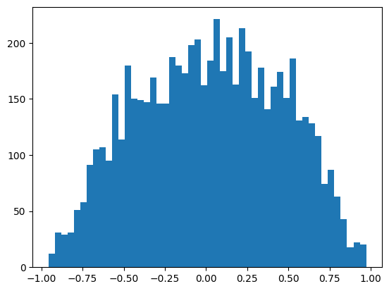
Let’s now take a quick look at the activation of the hidden layer (h).

plt.hist(h.view(-1).tolist(), 50);

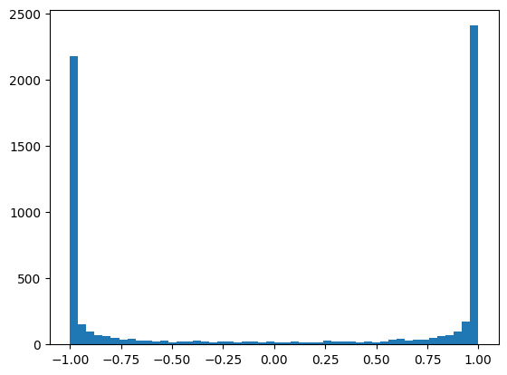
You can see that the outputs of the activation function live in the tail (i.e., [-1, 1]) of the tanh function. Remember that the tanh function is a squashing function which maps the values to the range of [-1, 1]. Why is this happening and why is this a problem?

Why is the tanh function saturated?

Activation state h is computed by applying the tanh function to the pre-activation state hpreact. Now, let’s take a look at the pre-activation state hpreact.

plt.hist(hpreact.view(-1).tolist(), 50);

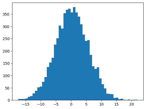
The input tensor to the tanh activation function is distributed in the range of [-15, 15]. And due to broad range of the input, the tanh function is saturated and thus producing outputs close to -1 or 1.

Why is this a problem?

Let’s bring back the tanh node of the Micrograd library that we have implemented in the previous post.

def tanh(self):
    x = self.data
    t = (math.exp(2 * x) - 1) / (math.exp(2 * x) + 1)
    out = Value(t, (self, ), 'tanh')

    def _backward():
        self.grad += (1 - t**2) * out.grad
    out._backward = _backward

    return out

As we compute the gradient of the loss with respect to the activation state h, we are running the chain rule of the derivative. The out.grad is the gradient from the loss function until the next layer of the activation function and we multiply it by the local gradient of the tanh function.

Since the tanh function is saturated (i.e., t is close to -1 or 1), we are effectively doing:

\[\nabla{h} = \begin{cases} (1 - 1^2) * \nabla{out} = 0, & t = 1 \\ (1 - (-1)^2) * \nabla{out} = 0, & t = -1 \\ \end{cases}\]

This means that the gradient of the loss with respect to the activation state h is 0 and thus the weights and biases are not updated during the training process.

This is known as the gradient saturation problem, which occurs when the gradients of a neural network become too small (vanishing gradient) or too large (exploding gradient), preventing effective learning during backpropagation. It primarily happens in deep networks with activation functions that squash their inputs into a limited range, leading to slow or stalled updates in the early layers.

The gradient saturation problem manifests in two main ways:

1. Vanishing Gradients: When activation functions like tanh or sigmoid are saturated (inputs are too large in magnitude), their derivatives become very close to zero. During backpropagation, these near-zero gradients are multiplied together, making the gradient signal progressively smaller as it moves through the layers. This makes it difficult for earlier layers to learn.

2. Exploding Gradients: Conversely, when weights are too large, the gradients can become extremely large during backpropagation, causing unstable updates and preventing the network from converging.

This is why proper weight initialization is crucial - it helps ensure that the activations and gradients remain in a reasonable range where learning can occur effectively. Now, let’s initialize W1 and b1 properly to resolve this issue.

Multiply b1 by a Small Number

Similar to the bias of the output layer, we can set the bias of the hidden layer close to zero.

b1 = torch.randn(n_hidden, generator=g) * 0.01 # Multiply `0.01` instead of `0` to introduce a small noise

Multiply W1 by a Small Number

W1 = torch.randn((n_embd * block_size, n_hidden), generator=g) * 0.01 # 0.02 in actual implementation

Multiplying W1 by a 0.1 has scaled both the pre-activation (hpreact) and the activation (h) state.

Now, the distribution of pre-activation state is centered around zero with standard devition of approximately 1.0.

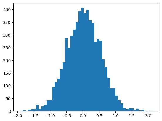
And as a result, we have a stable activation state which the distribution no longer located in the tail of the tanh function.

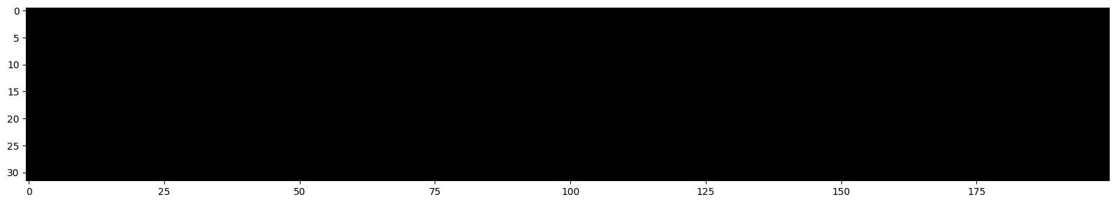
Also, let’s take a closer look at the neuron per training set’s mini-batch:

plt.figure(figsize=(20, 10))
plt.imshow(h.abs() > 0.99, cmap='gray', interpolation='nearest')

Random Initialization

Scaled by 0.1

Scaled by 0.2

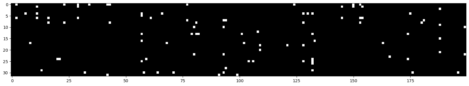
Visualization above shows the value of the nueron after the activation (tanh can have [-1, 1] as the output range) per 32 mini-batches. Neurons with absolute value greater than 0.99 are highlighted in gray. If there is a neuron that is completely white, it means that the neuron is dead thus does not contribute to the training.

What is the Optimal Scaling Factor?

So far, we have multiplied relatively small scaling factor (i.e., 0.01, 0.2) to the weights and biases. But what is the optimal scaling factor?

Let’s take a look at one last example before we dive into popular weight initialization methods.

x = torch.randn(1000, 10)
w = torch.randn(10, 200)
y = x @ w

print('x.mean:', x.mean(), 'x.std:', x.std())
print('y.mean:', y.mean(), 'y.std:', y.std())

plt.figure(figsize=(20, 5))
plt.subplot(121)
plt.hist(x.view(-1).tolist(), 50, density=True);
plt.subplot(122)
plt.hist(y.view(-1).tolist(), 50, density=True);

x.mean: tensor(-0.0034) x.std: tensor(0.9939)
y.mean: tensor(0.0080) y.std: tensor(3.0881)

We created tensors x and w using torch.randn which returns a tensor filled with random numbers from the normal distribution with mean 0 and variance 1. Multiplying x by w results in a tensor y with mean 0 and variance 3.

Although the mean stays at 0, the variance of both tensors get propagated through the multiplication, thus expanding the distribution of the output tensor y.

As we have seen that maintaining the gaussian distribution across the layer is crucial for stable training, we can multiply the weights by a scaling factor of $\frac{1}{\sqrt{fanin}}$ to keep the variance of the output tensor y around 1.

x = torch.randn(1000, 10)
w = torch.randn(10, 200) / (10**0.5)
y = x @ w

print('x.mean:', x.mean(), 'x.std:', x.std())
print('y.mean:', y.mean(), 'y.std:', y.std())

x.mean: tensor(-0.0089) x.std: tensor(1.0125)
y.mean: tensor(-0.0003) y.std: tensor(1.0168)

For Multi-Layer Perceptron (MLP), we can have a deep neural network with stacked non-linear activation functions. The weight initialization techniques that we will be discussing in the next section ensures that the activation state does not explode nor vanish during the training process by multiplying the appropriate scaling factor to the weights.

Kaiming He Initialization

Kaiming He Initialization was first propsed in Delving Deep into Rectifiers:Surpassing Human-Level Performance on ImageNet Classification.

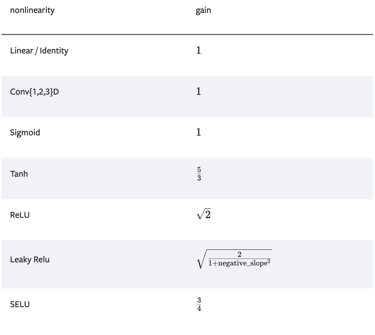
Kaiming He Initialization was specifically designed for ReLU and its variant activation functions which introduce asymmetry by zeroing out the negative values (you can still use it for squashing functions like tanh or sigmoid as long as the gain is configured accordingly). The generalized formula is as follows:

Normal Distribution (Kaiming Normal)

\[\text{W} \sim \mathcal{N}(0, \frac{gain^2}{\text{fan_mode}})\]

Where:

• $\text{gain}$: a scaling factor that depends on the activation function.
• $\text{fan_mode}$: fan-in (for mode=’fan_in’) or fan-out (for mode=’fan_out’).

Uniform Distribution (Kaiming Uniform)

\[\text{W} \sim \mathcal{U}(-\frac{gain \cdot \sqrt{6}}{\sqrt{\text{fan_mode}}}, \frac{gain \cdot \sqrt{6}}{\sqrt{\text{fan_mode}}})\]

Xavier Initialization

Xavier Initialization was first proposed in Understanding the difficulty of training deep feedforward neural networks.

Xavier initialization assumes that the variance of the activations should remain constant across the layers. It is best suited for the squashing functions like tanh or sigmoid that are symmetric around zero.

Normal Distribution (Xavier Normal)

\[\text{W} \sim \mathcal{N}(0, \frac{gain^2}{\text{fan_in} + \text{fan_out}})\]

Uniform Distribution (Xavier Uniform)

\[\text{W} \sim \mathcal{U}(-\frac{gain \cdot \sqrt{6}}{\sqrt{\text{fan_in} + \text{fan_out}}}, \frac{gain \cdot \sqrt{6}}{\sqrt{\text{fan_in} + \text{fan_out}}})\]

PyTorch Documentation: Initialization

Let’s take a look at PyTorch’s nn.init documentation to better understand the mathematical equations.

If we were to initialize the weights for tanh activation function using Kaiming Normal, we should use torch.nn.init.kaiming_normal_:

Documentation introduces API below:

torch.nn.init.kaiming_normal_(tensor, a=0, mode='fan_in', nonlinearity='leaky_relu', generator=None)

Parameters:

• tensor (Tensor): an n-dimensional torch.Tensor
• a (float): the negative slope of the rectifier used after this layer (only used with leaky_relu)
• mode (str): either fan_in (default) or fan_out. Choosing fan_in preserves the magnitude of the variance of the weights in the forward pass. Choosing fan_out preserves the magnitudes in the backwards pass.
• nonlinearity (str): the non-linear function (nn.functional name), recommended to use only with relu or leaky_relu (default).
• generator (Optional[Generator]): the torch Generator to sample from (default: None)

Parameters mode and nonlinearity are the same as the ones we have discussed in the previous mathematical equations.

Example: Kaiming Normal for tanh

In PyTorch, we can initialize the weights for tanh activation function using Kaiming Normal by calling:

torch.nn.init.kaiming_normal_(W1, nonlinearity='tanh') # default mode is `fan_in`

For our example, we can use the following code to initialize the weights for the hidden layer:

W1 = torch.randn((n_embd * block_size, n_hidden), generator=g) * ((5/3) / (n_embd * block_size)**0.5)

Conclusion

This post explored why proper weight initialization is crucial for training neural networks effectively. We demonstrated how random initialization can be problematic, often leading to extreme loss values due to gradient saturation in the network.

We found that a key solution lies in carefully scaling weights and biases to maintain a distribution centered around zero with a standard deviation of 1. This approach helps prevent both gradient explosion and vanishing gradient problems. We examined two popular methods - Kaiming He and Xavier Initialization - which provide mathematically sound approaches for determining optimal scaling factors based on the choice of activation function.

While these initialization techniques work well for many architectures, they aren’t perfect solutions for all scenarios. Modern deep neural networks have grown increasingly complex, sometimes requiring more sophisticated initialization strategies. Fortunately, architectural innovations like ResNets and techniques like batch normalization have helped address these challenges, making deep networks more trainable regardless of initialization.